Face Morphing

Introduction

In this project, I explored face morphing and the concept of an “average face” over a population. I used an image of myself and morphed it into different images of other people and into average face geometry.

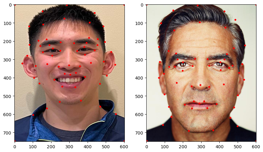
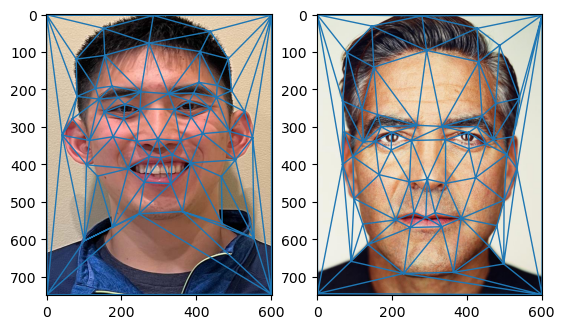
Part 1: Defining Correspondences

To morph one face into another, the images need to be aligned in terms of key facial features.

I manually selected corresponding points on both images and then used those points to define a triangulation. With corresponding triangles, I could compute transforms to warp each face to a shared geometry.

I implemented point selection with ginput from matplotlib, and used Delaunay triangulation to avoid overly skinny triangles. I ran triangulation on the average of the landmark points so the same triangulation could be used for both images.

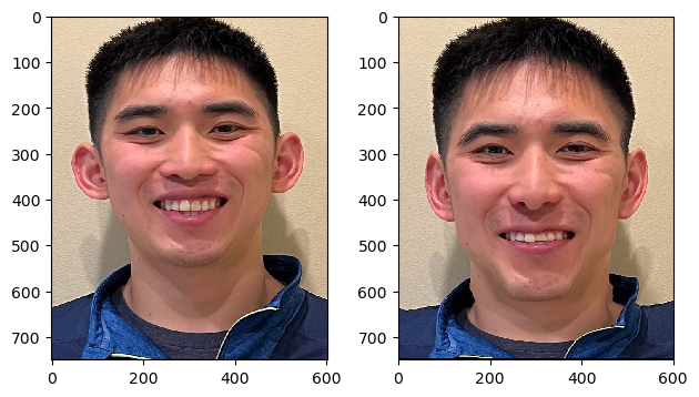
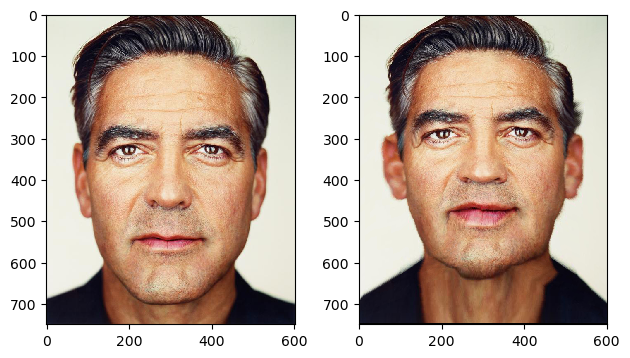
Part 2: Computing the Mid-Way Face

After defining correspondences and triangulation, I computed the mid-way face between two people.

This is done by warping both faces into the average keypoint configuration and then averaging the two warped images across color channels. The warping uses affine transforms between corresponding triangles with inverse warping.

Here is the mid-way result between my face and George Clooney’s face:

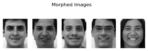
Part 3: The Morph Sequence

Using a similar pipeline as Part 2, I produced a smooth morph sequence between two faces.

At each frame, I used linearly interpolated keypoints between the two faces and inverse warped each source image into that intermediate geometry, then blended colors according to the interpolation factor.

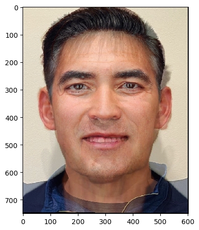
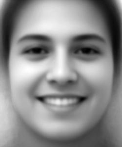
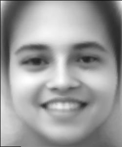
Part 4: The Mean Face of a Population

I computed the mean face of a population by averaging keypoints over all faces, warping each face into that mean geometry, and then averaging the warped images.

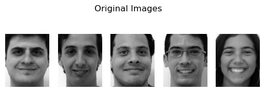
The dataset used was the FEI Face Database, using spatially normalized frontal images.

Examples from the dataset and their warped versions:

Mean face result:

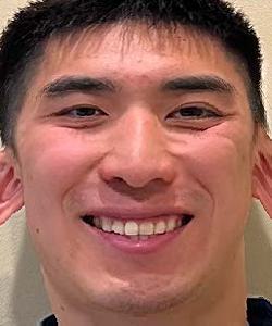
I also warped my face to average geometry and warped the average face toward my geometry:

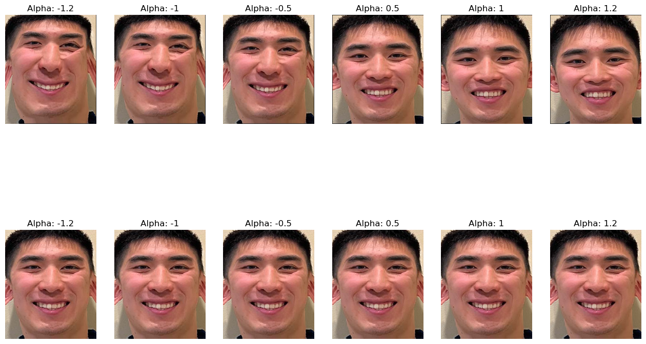
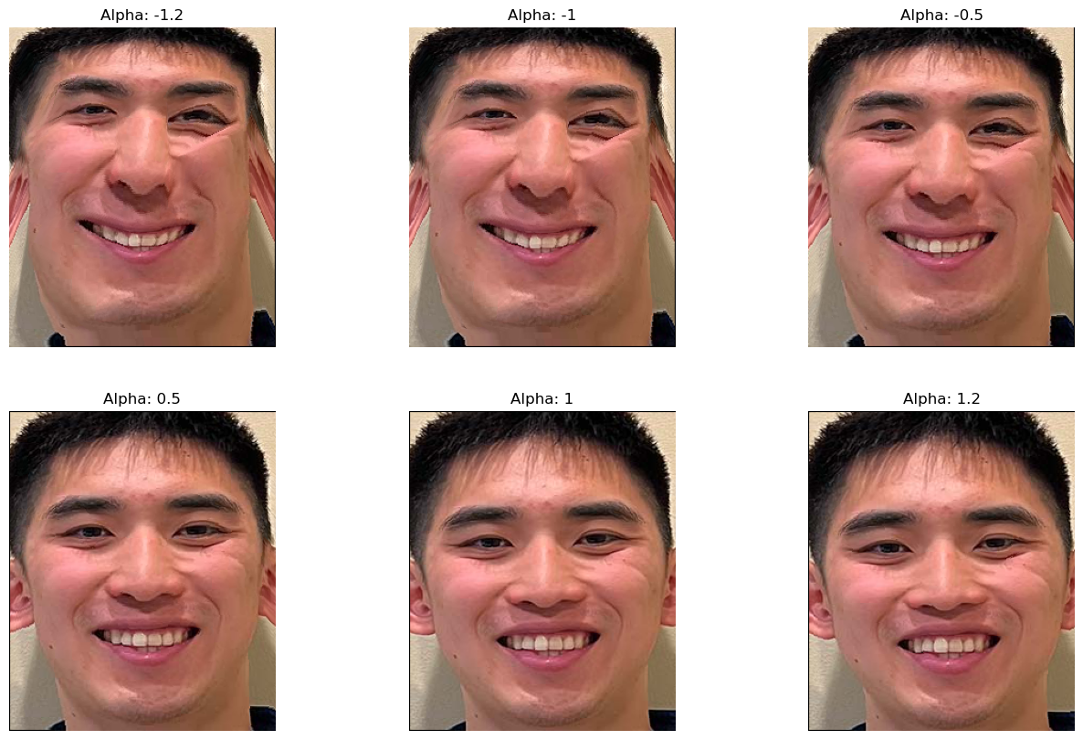
Part 5: Caricatures

I extrapolated from population averages to create caricatures.

Using the mean from Part 4:

\[\text{extrapolated} = \text{average} + \alpha \cdot \text{img}\]

where operations are performed per pixel and \(\alpha\) controls extrapolation strength.

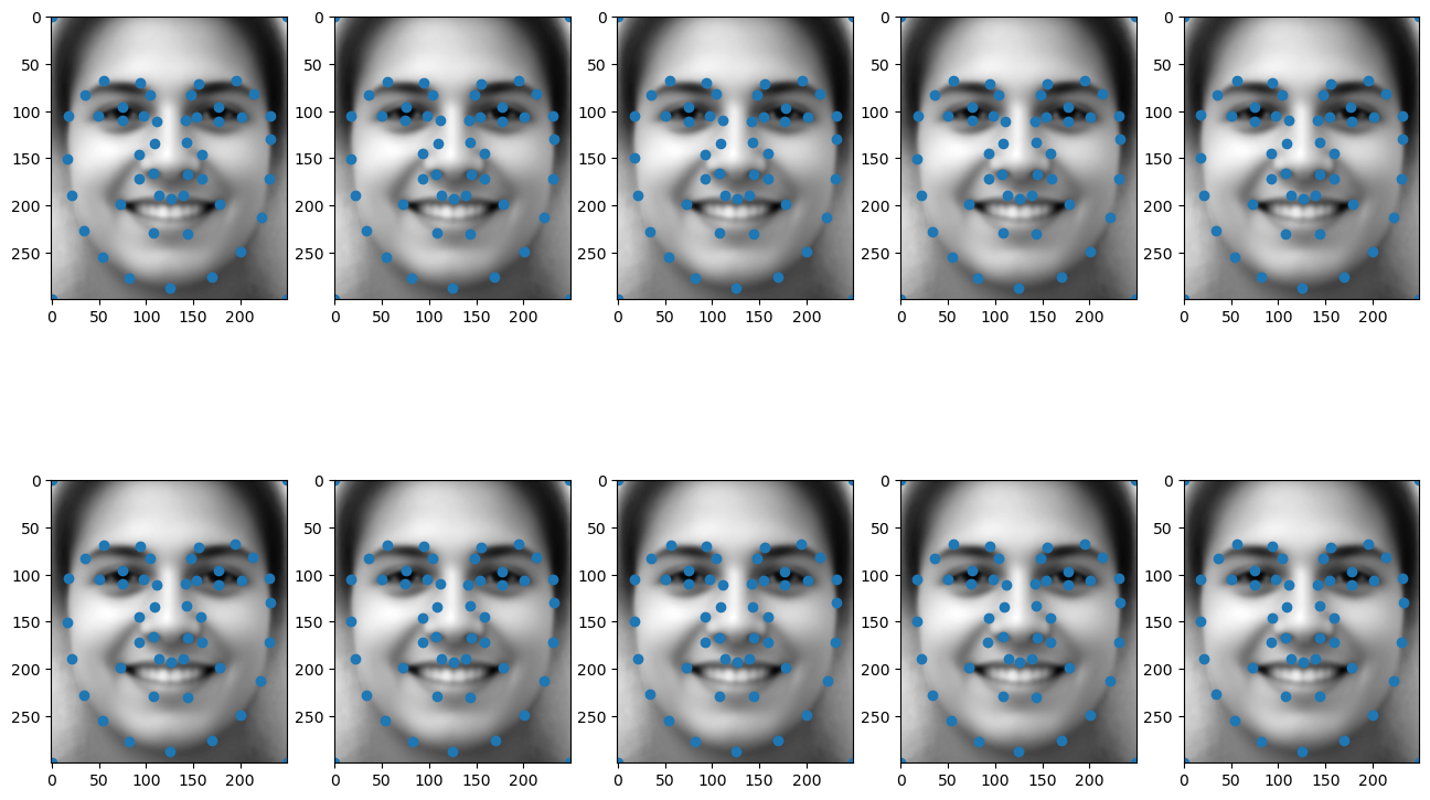
Bells and Whistles: PCA Basis

I constructed a PCA basis for keypoints across the dataset to capture the major modes of variation.

After zero-centering keypoints for PCA, I added back the mean for visualization on the average face. Many keypoints appear similar because the dataset is already fairly well aligned.

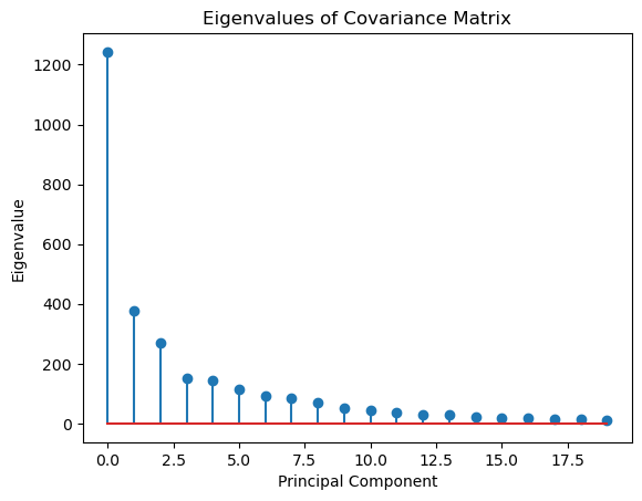
I also visualized eigenvalues to inspect how variance is distributed across principal components.

Using PCA basis vectors, I generated caricature-style transformations:

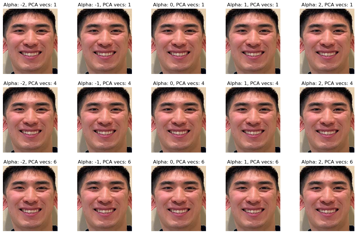
Compared with the original caricatures, PCA-based caricatures appear less extreme in this setup: