Fun with Filters and Frequencies

Part 1: Fun with Filters

Finite Difference Operator

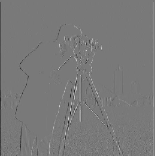
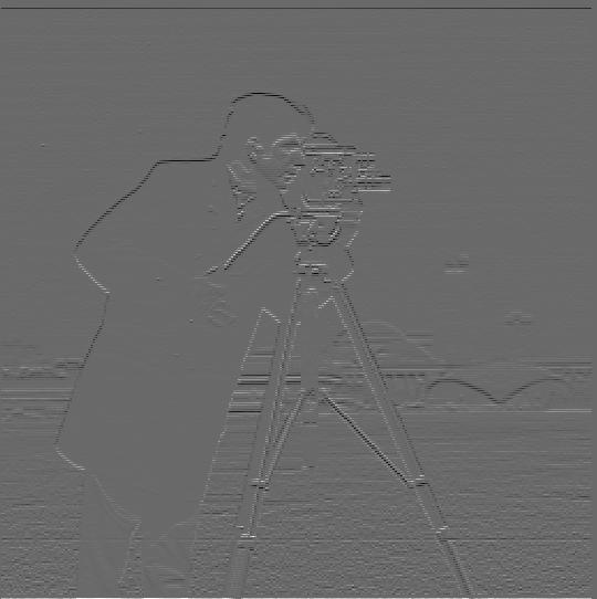
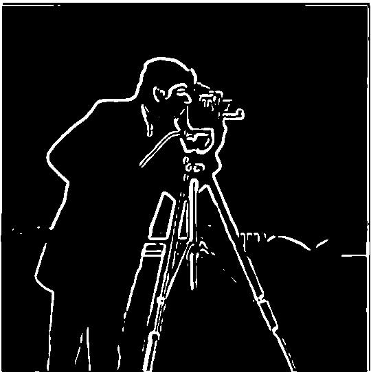
A common task in image processing is finding the edges in an image along both the horizontal and vertical directions. This is often done by computing the gradients of the image along the x and y directions. This can be simply done by convolving the image with simple kernels that approximate the derivative of the image using finite differences. These kernels are simply taking the difference between two consecutive pixels in the image as an approximation of the true derivative.

\[\text{Gradient in x direction: } \matrix{D_x} = \begin{bmatrix} 1 -1 \end{bmatrix}\] \[\text{Gradient in y direction: } \matrix{D_y} = \begin{bmatrix} 1 \ -1 \end{bmatrix}\]

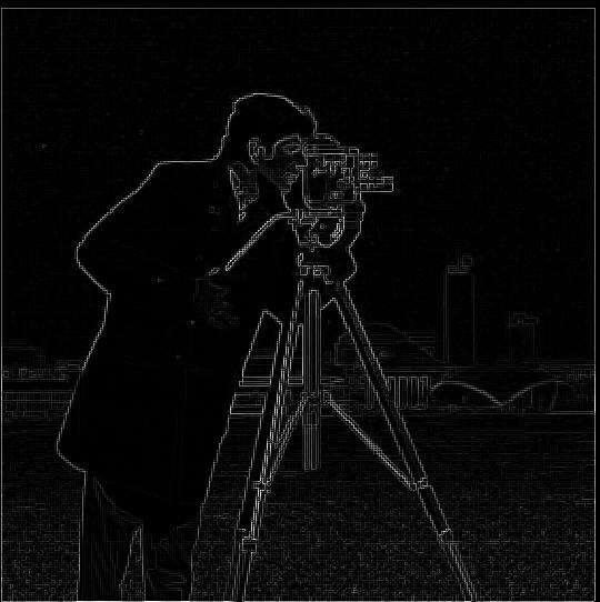
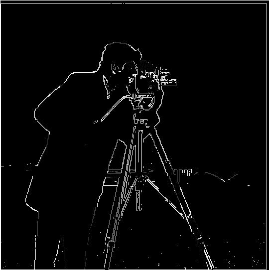
We can also compute the magnitude of the gradient by taking the square root of the sum of the squares of the gradients in the x and y directions to visualize the edges in the image. In order to remove some of the noise, we also can threshold the gradient magnitude to get a clearer picture of the edges in the image.

Derivative of Gaussian (DoG Filter)

We can also smooth out our gradient magnitude edges by smoothing image first using a Gaussian filter. Convolving our image with a Gaussian filter gives us a cleaner picture of the edges. When we thresholded, we could tell we were only displaying the stronger edges and there was less noise in the image. However, there were also some gaps in the edges that we did have due to this thresholding. We can see in the smoothed version that the edges are more continuous and there are less gaps in the edges.

Due to the linear nature of convolutions, we can also compute this smoothed gradient magnitude using only one filter instead of two. This filter is known as the Derivative of Gaussian (DoG) filter and works by convolving the Gaussian with the finite difference operators first. Since these are much smaller than the image, we can convolve the Gaussian with the finite difference operators first and then convolve the result with the image to get the same result in less time.

Part 2: Fun with Frequencies

Image Sharpening

Another common task in image processing is image sharpening. A simple way we can accomplish this is by adding high-frequency components back into the image.

We can get the high-frequency portions by subtracting the blurred image from the original image. This gives us high-frequency components that we can add back with an enhancement factor to sharpen the image.

Combining these operations into one filter gives us the unsharp mask filter. The process is outlined below for two example images:

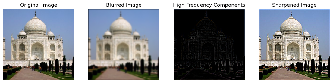
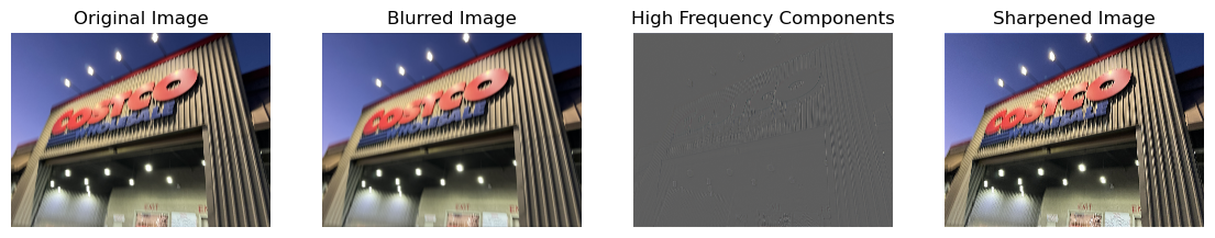
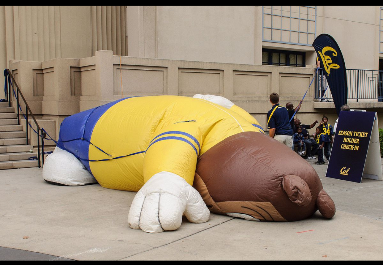
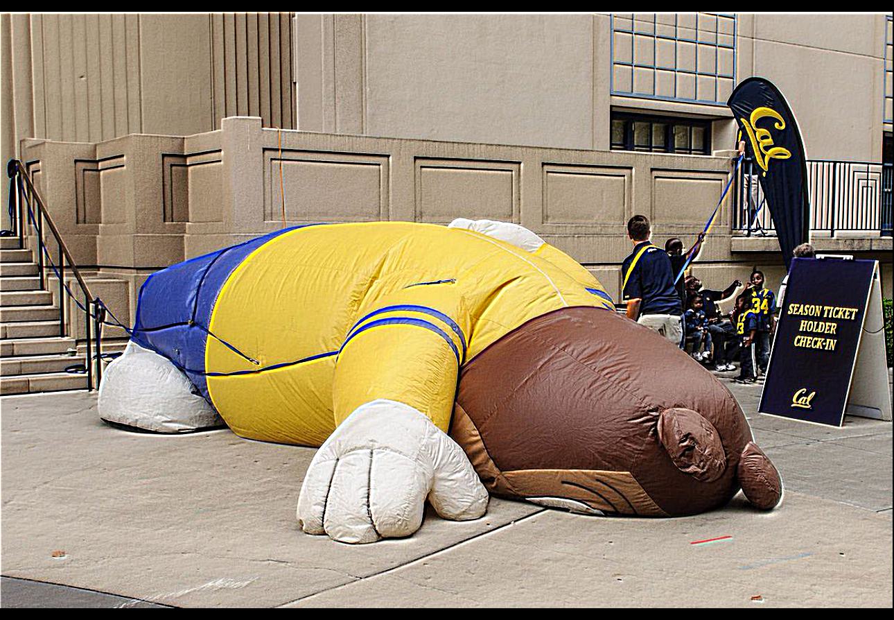
Here are some results from testing this filter on several blurry images.

From these examples, we can see that the unsharp mask filter does a good job of enhancing some higher-frequency components. It does particularly well with lines in building structures.

However, it is far from perfect as an unblurring filter since it only enhances edges already present in the image and cannot recover lost details.

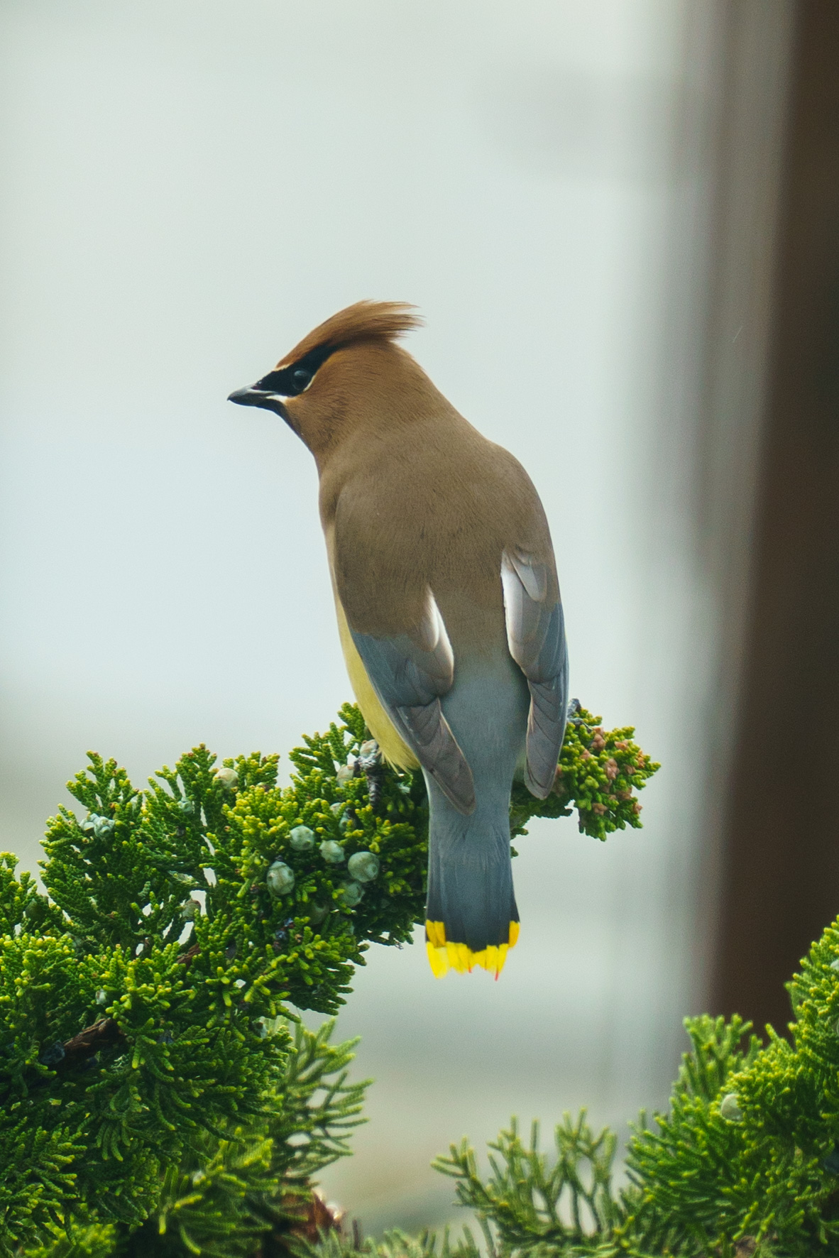
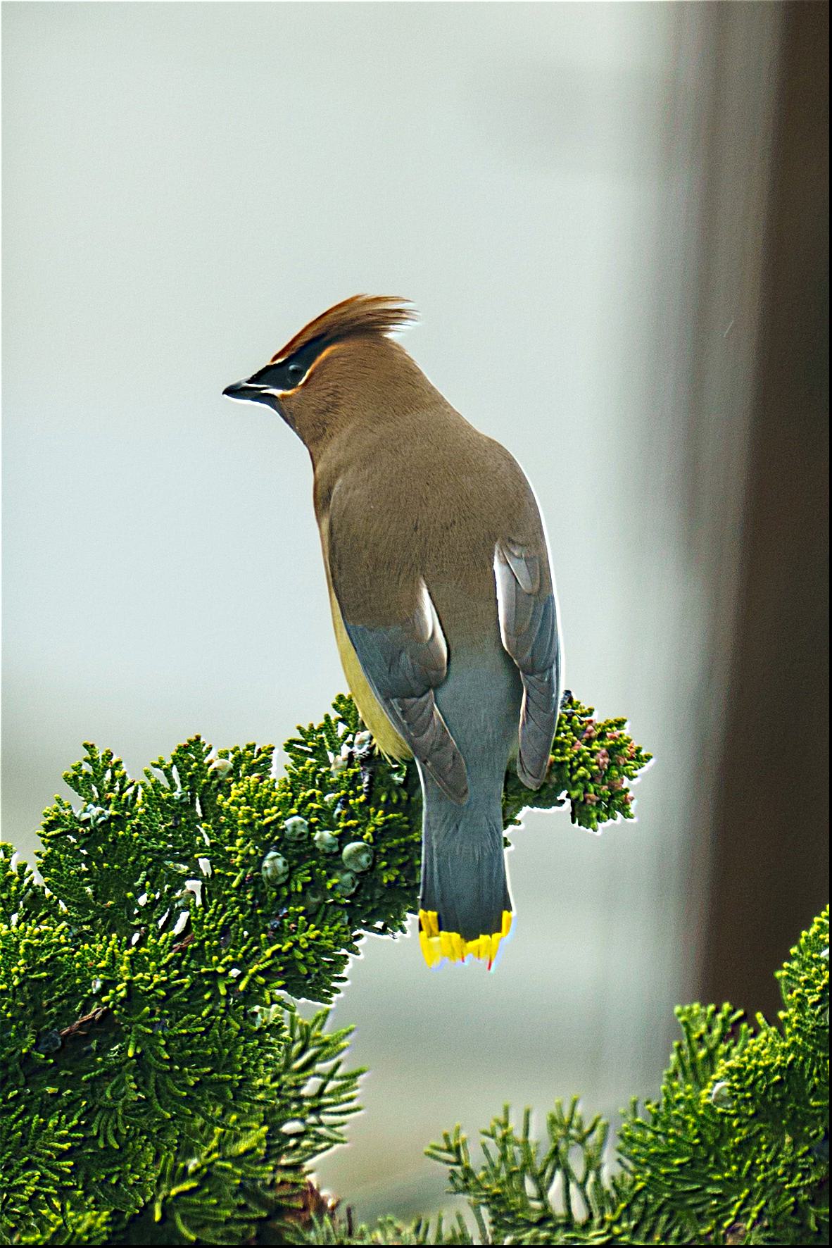
For fun, this is what happens when we apply the unsharp mask filter to a blurred and re-sharpened image:

This image was already decently sharp. I then blurred and re-sharpened it. The result is an image of Oski with even sharper edges than the original.

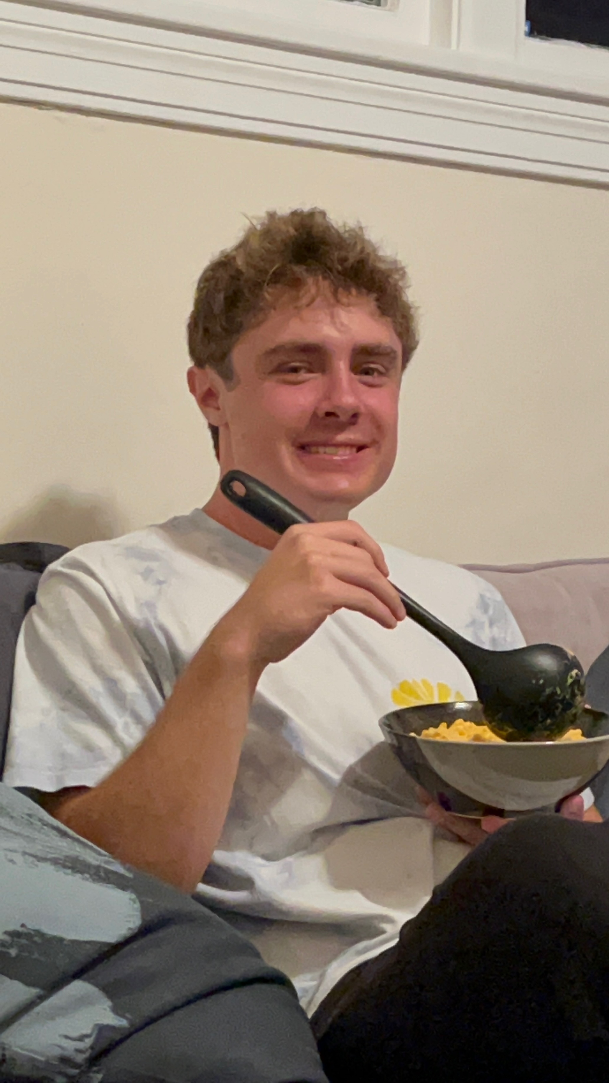
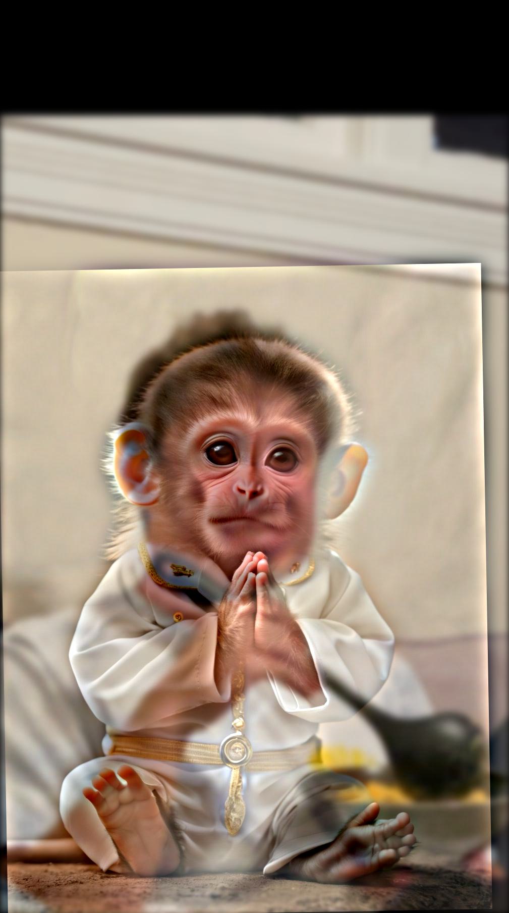
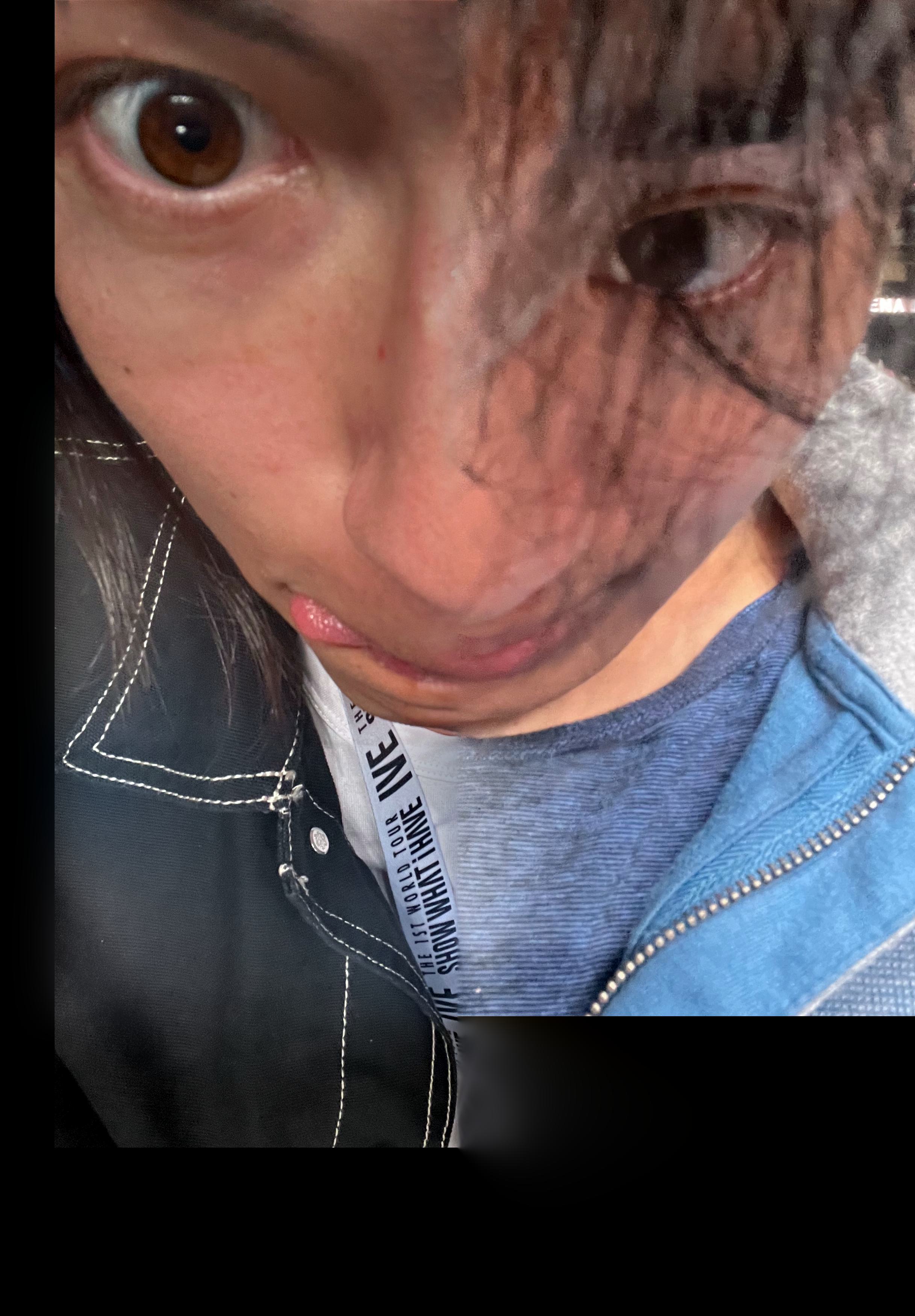
Hybrid Images

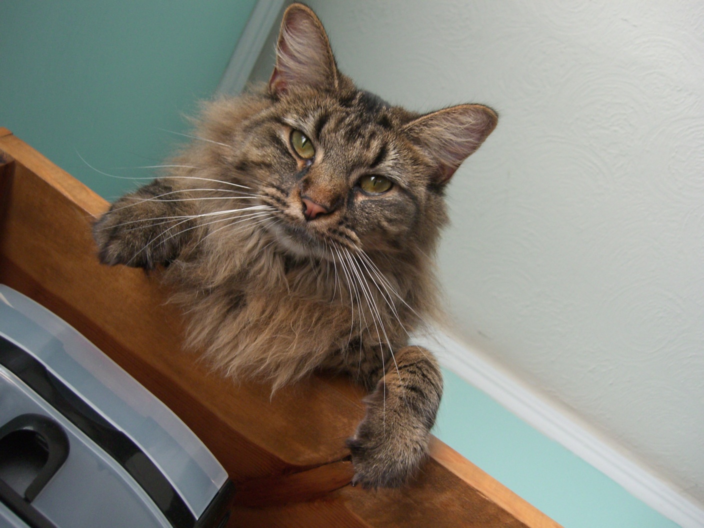
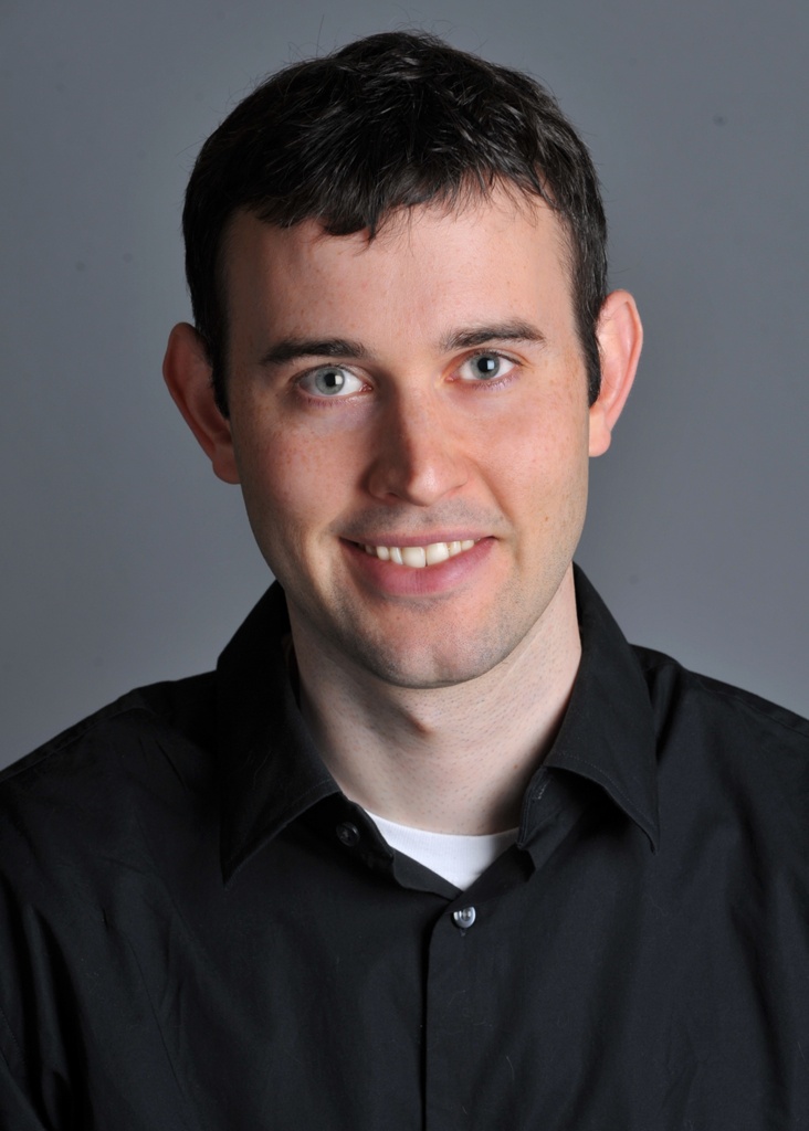
In this section, I created hybrid images by combining low-frequency components of one image with high-frequency components of another image.

Since humans perceive low frequency much better than high frequency, up close we see mostly the low-pass image. From farther away, we can see elements of the high-pass image.

As before, I get low-pass components by Gaussian blurring. I get high-pass components by subtracting the low-pass filtered image from the original image. Then I average the two filtered images to produce the hybrid image.

We can control the amount of high-frequency content by adjusting the Gaussian sigma. Higher sigma changes how much frequency content is retained.

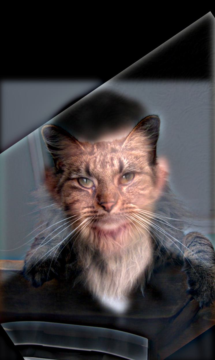
Before hybridizing, I aligned the two images by matching points and resizing to the same dimensions.

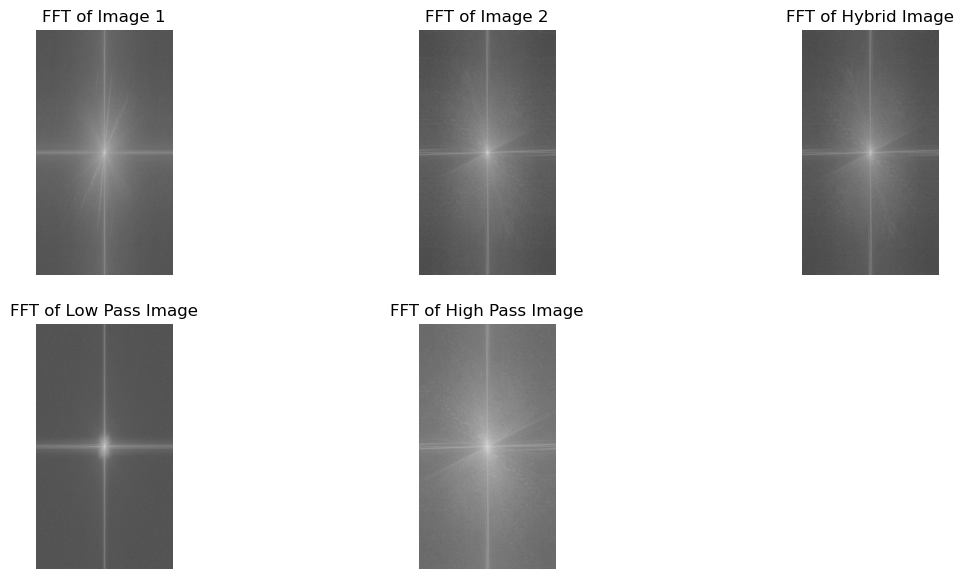
We can visualize frequency response by taking the Fourier transform and plotting its magnitude.

As shown below, the hybrid keeps low-frequency portions of image 1 and high-frequency portions of image 2.

Here are other hybrid-image examples:

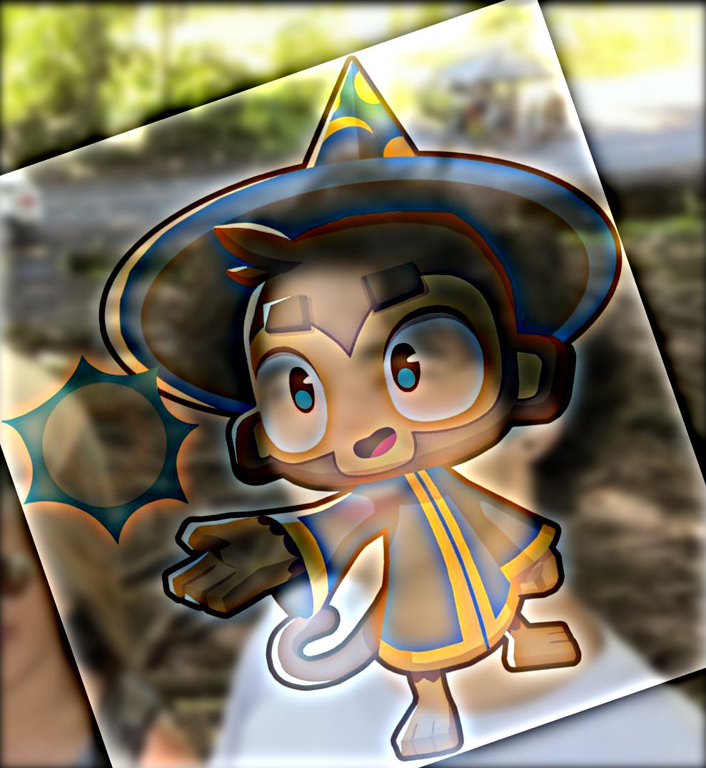
This last image did not turn out great, likely because shapes and color schemes of the two source images were too different. It mostly looked like one image with a slight ghost of the other.

Multi-resolution Blending

Another common task in image processing is blending two images together. If we simply splice images, we get a harsh seam between them.

Multiresolution blending smooths this seam by blending at multiple resolutions and recombining.

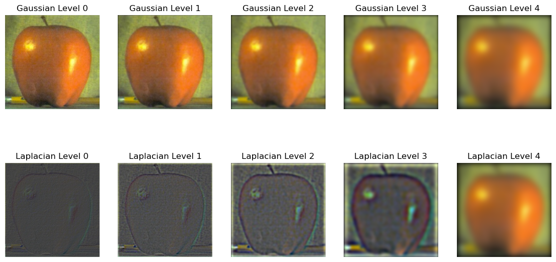
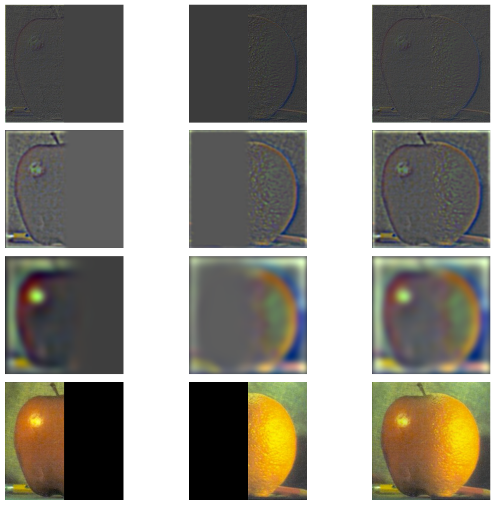
Gaussian and Laplacian Stacks

To separate images into resolutions, I used Gaussian and Laplacian stacks. These decompose images into different frequency bands for later combination.

Unlike the Gaussian pyramid from project 1, here I built Gaussian stacks by applying Gaussian kernels with increasing sigma values. I then got Laplacian stacks by subtracting adjacent Gaussian levels.

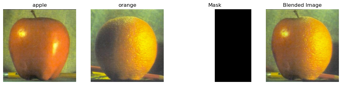
Implementing Multi-resolution Blending

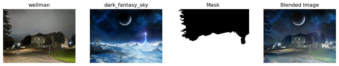
Following Burt and Adelson, I blended two images by creating Gaussian and Laplacian stacks for both images, plus a Gaussian stack for the mask to smooth jagged edges from a simple spline blend.

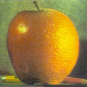
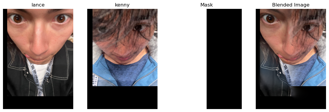
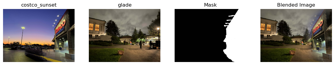
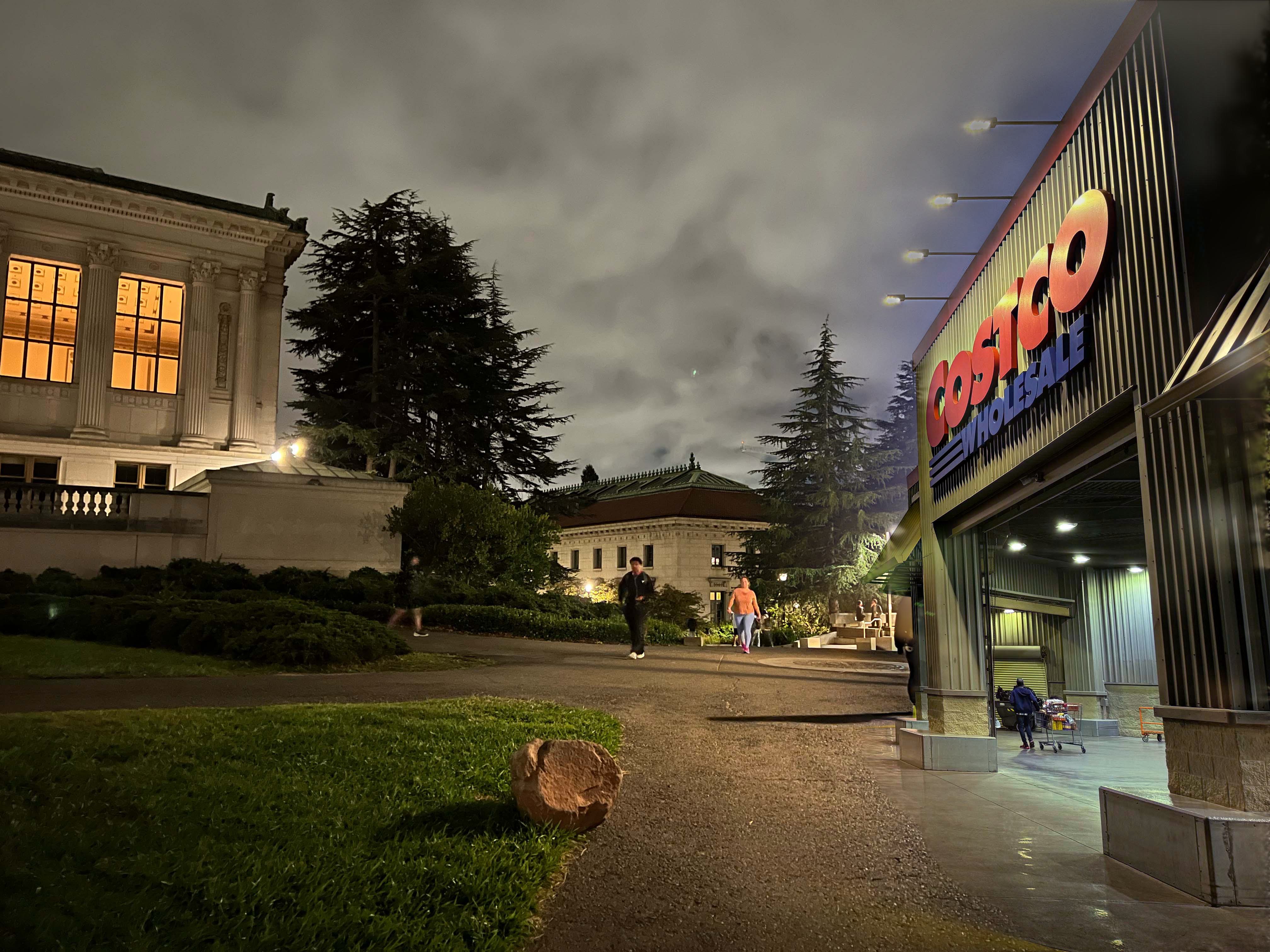
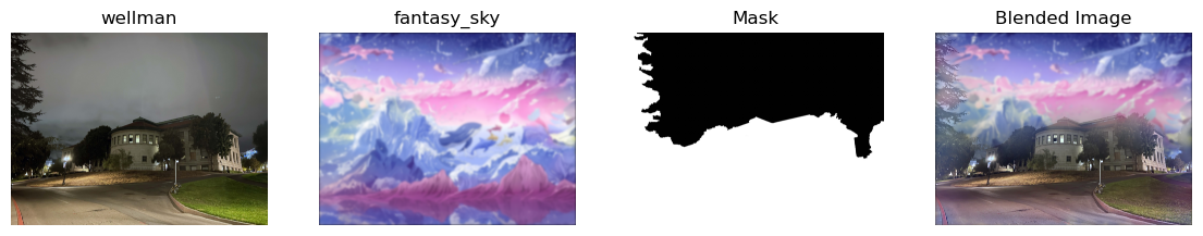
Here are my blending results:

Takeaways

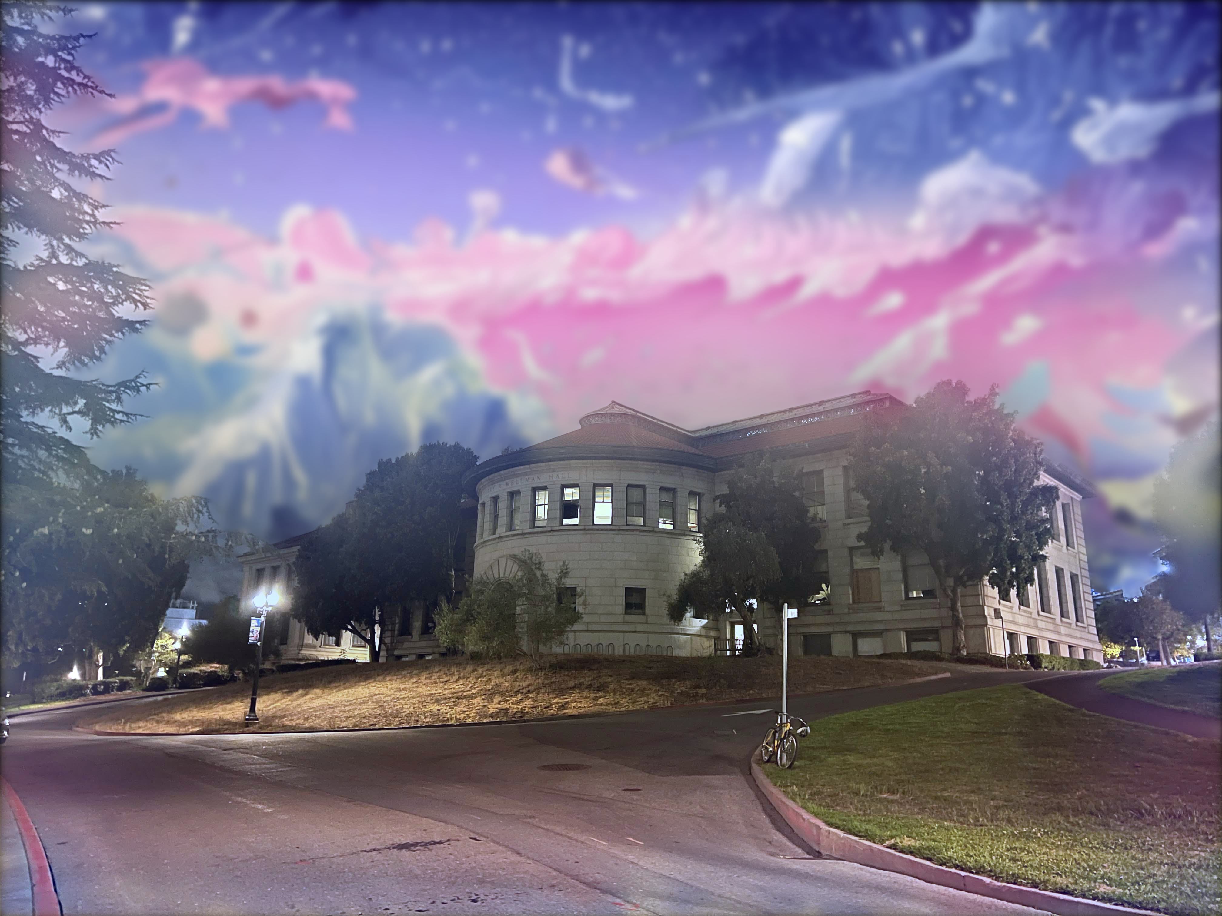
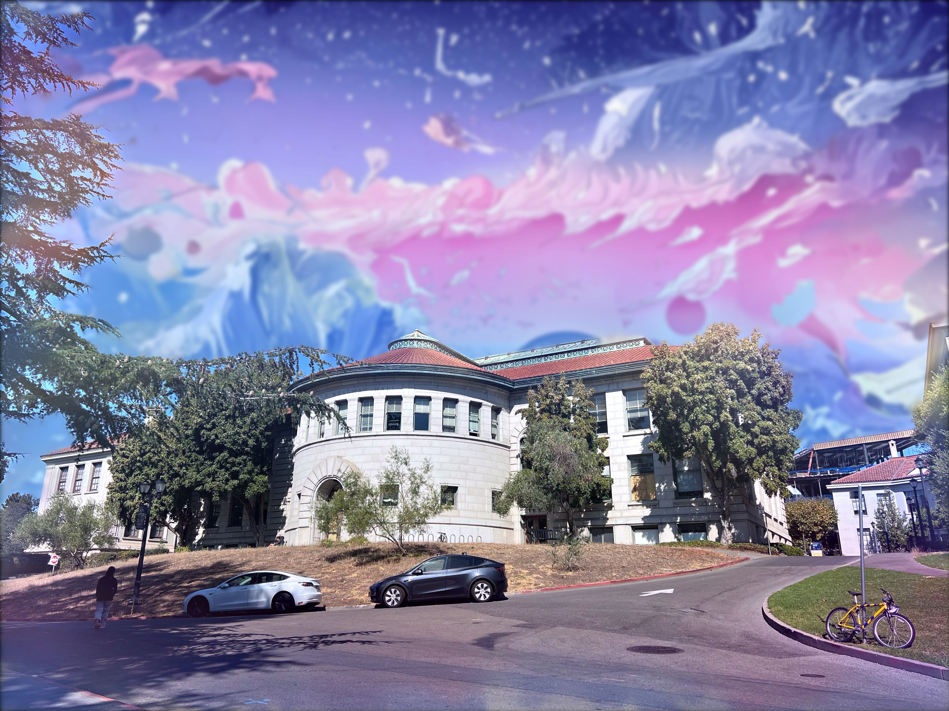
After blending with a basic vertical mask, I first tried inserting an object into an image with an irregular mask. That did not work well due to color mismatch and different fields of view.

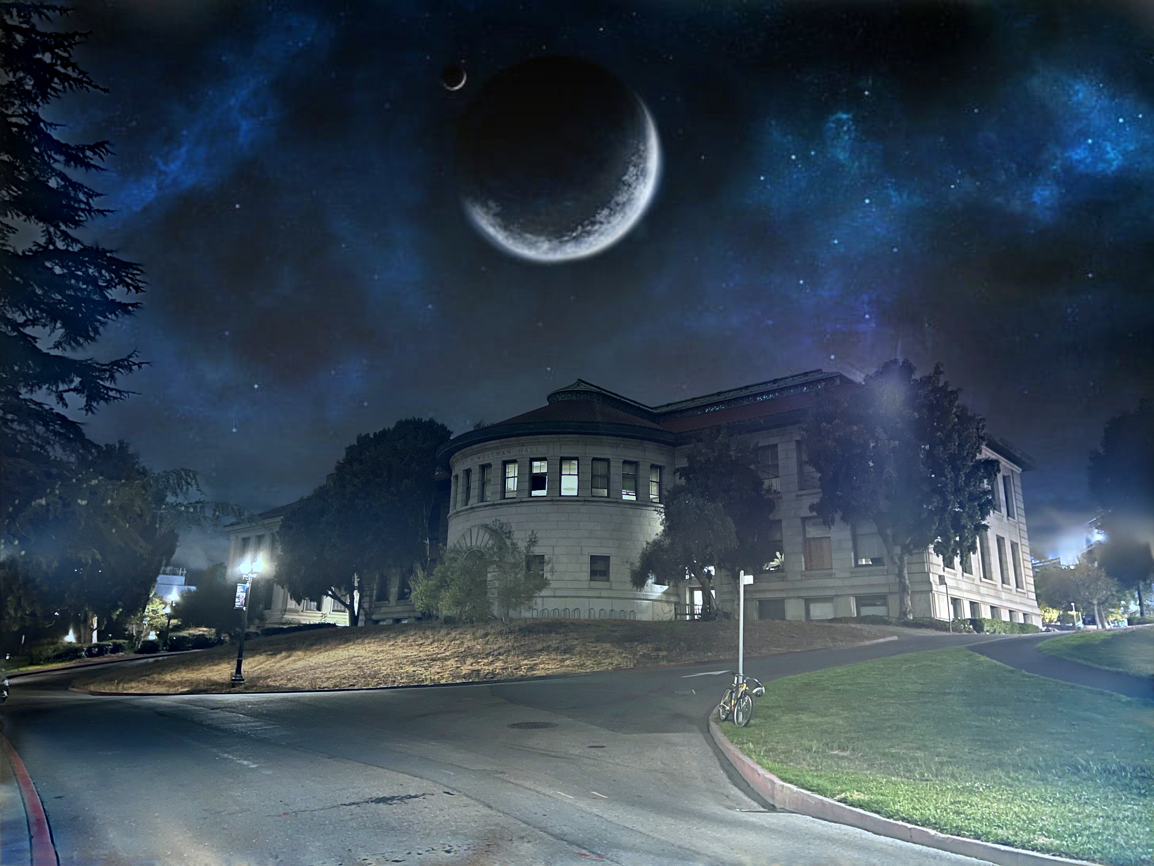
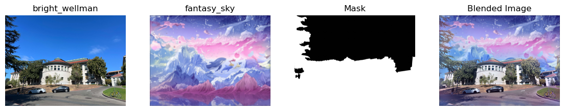
I then tried blending just the sky, which still looked slightly irregular due to color differences and scene shadows. Finally, I used skies with closer shading and got better blends with the building.

I drew irregular masks by hand in Photoshop. Jagged mask edges became unnoticeable in the final output because the Gaussian stack blurred the mask boundaries.

My main takeaway is how much simple operations can improve and manipulate images. More advanced methods would likely do better, but I was happy with the results from this pipeline and found it very interesting how far Gaussian-based filtering can go.