CS 180

Neural Radiance Fields

By Evan Chang · CS 180 Final Project

Tech: Python, NumPy, PyTorch, NeRF, Positional encoding, Volume rendering

Introduction

For my final project, I implemented a Neural Radiance Field (NeRF) model to render 3D scenes. NeRF is a method that can render novel views of a scene by learning a continuous function that maps 3D coordinates to RGB and density values. This allows the generation of photorealistic images of 3D scenes from a small number of images. The model is trained on a dataset of images and corresponding camera poses, and can then be used to render novel views of the scene. I based much of this project on the original NeRF paper.

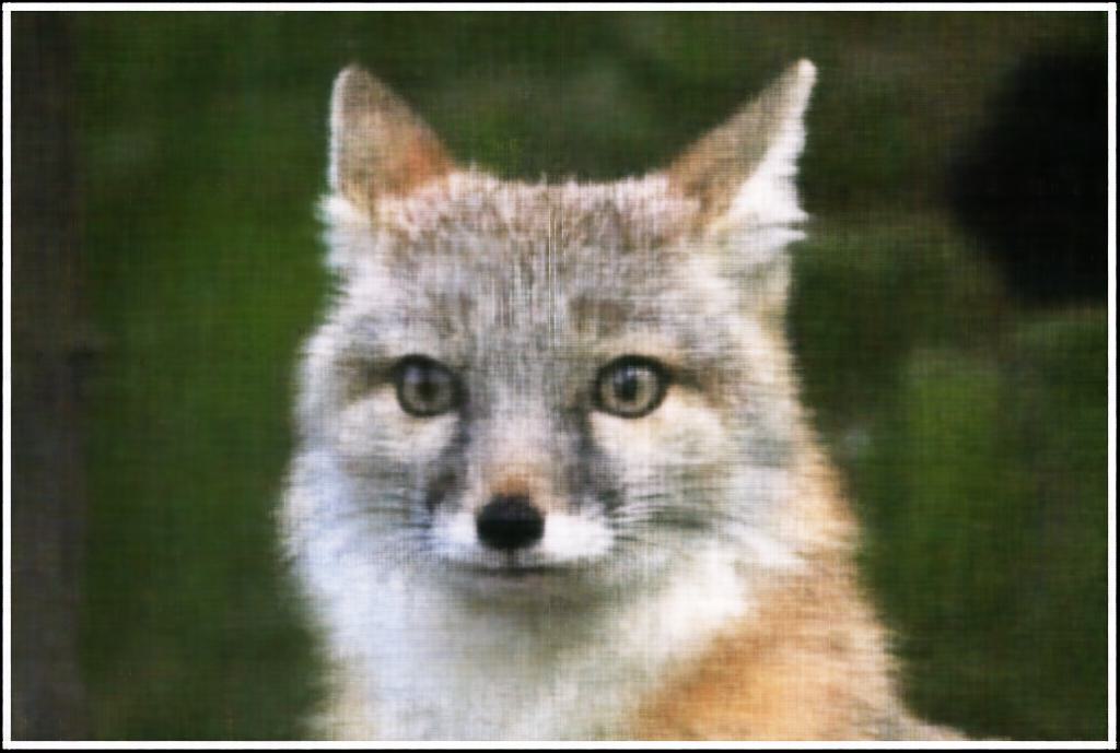
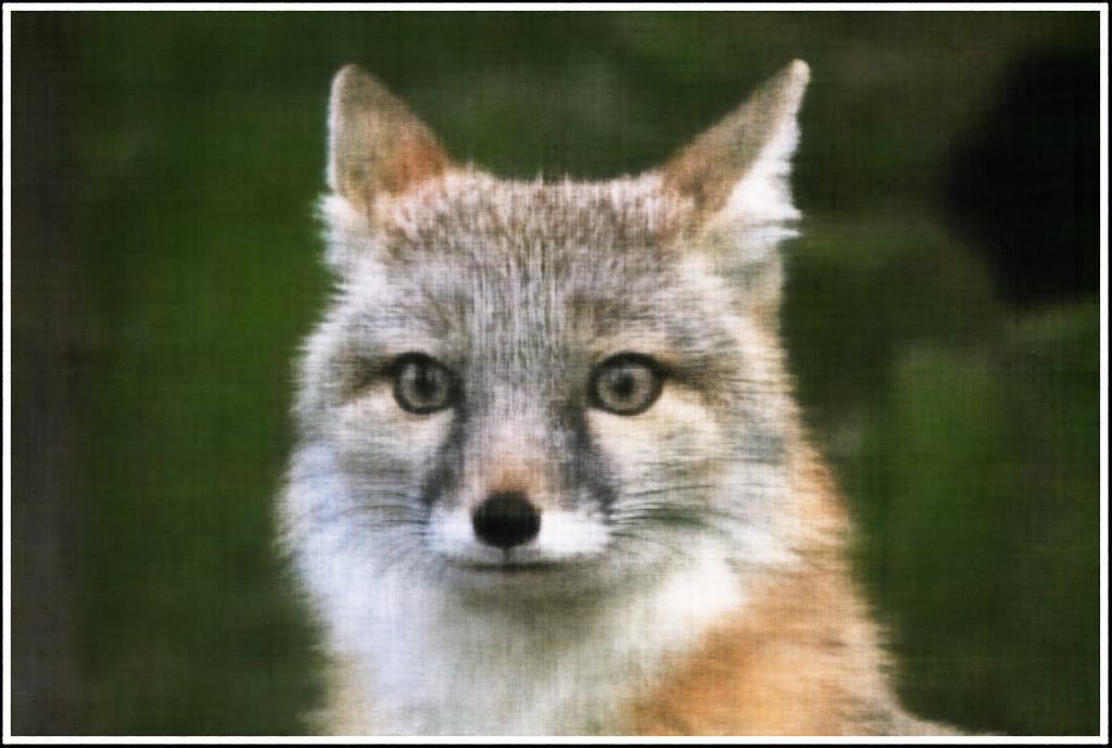
Part 1: Fitting a Neural Field to a 2D Image

In the first part of this project, I started by building intuition for Neural Fields with a 2D version of the model. The goal was to fit a Neural Field to 2D images without modeling radiance. Our system simplifies to implementing a field \(F: {u, v} \rightarrow {r, g, b}\) that maps 2D pixel coordinates to RGB values. We can do this with a multilayer perceptron (MLP) using sinusoidal positional encoding (PE) that takes a 2D input and outputs a 3D value (pixel color).

Model Architecture

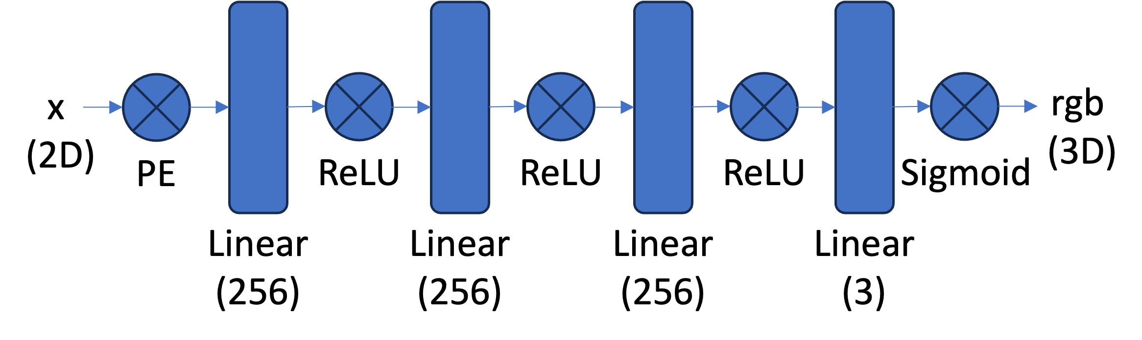
The network is composed of fully connected layers with ReLU activations. One of the most important parts of this architecture is sinusoidal positional encoding (PE). This operation expands the dimensionality of the input by adding sinusoidal functions at different frequencies. That helps the model learn higher-frequency patterns in the data based on the maximum frequency level \(L\) we choose.

\[ PE(x) = \{x, \sin(2^0\pi x), \cos(2^0\pi x), \sin(2^1\pi x), \cos(2^1\pi x), \ldots, \sin(2^{L-1}\pi x), \cos(2^{L-1}\pi x)\} \]

Our overall architecture is shown below. We use a Sigmoid activation at the end to constrain outputs to \((0, 1)\), matching valid pixel color ranges.

Dataloader

The first step in training a 2D Neural Field is generating training data. Because the images are too high resolution to use all pixels every step, we randomly sample \(N\) pixels per training iteration. The dataloader returns both the \((N \times 2)\) pixel coordinates and corresponding \((N \times 3)\) RGB values. These are the model inputs and supervision targets. I also normalized both before feeding them into the network.

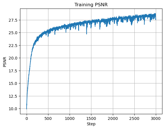
Training

I trained with mean squared error (MSE) loss and Adam with learning rate \(0.01\). The model runs for \(2000\) iterations with batch size \(10{,}000\) and max frequency level \(L=10\). Instead of reporting MSE directly, I use PSNR, which is standard for image reconstruction quality. For images normalized to \([0,1]\), PSNR is:

\[ PSNR = 10 \cdot \log_{10}\left(\frac{1}{\text{MSE}}\right) \]

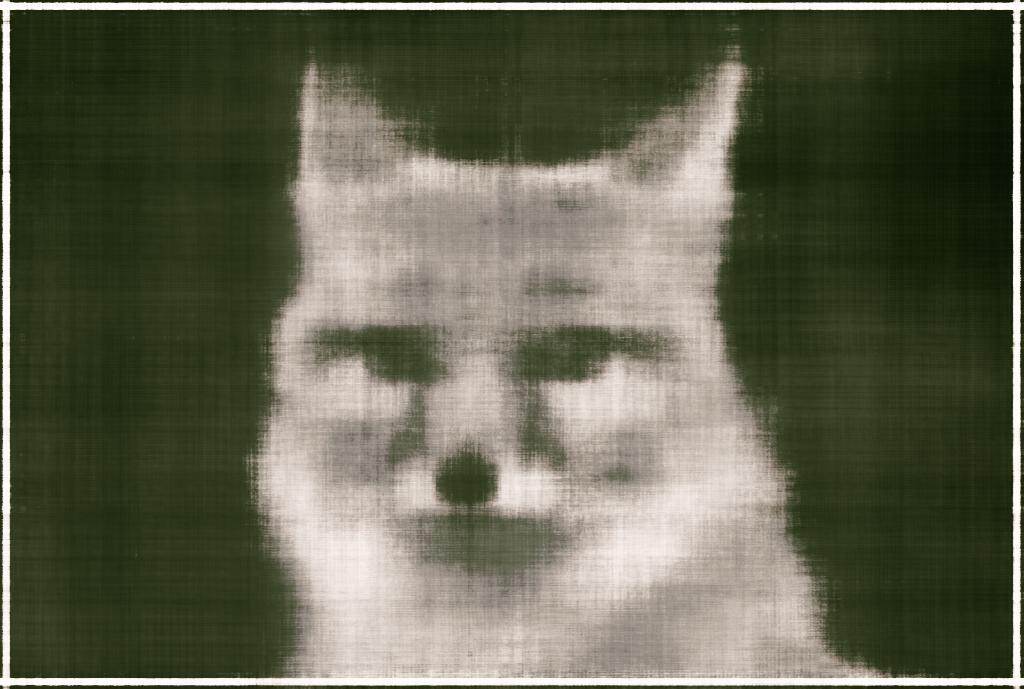
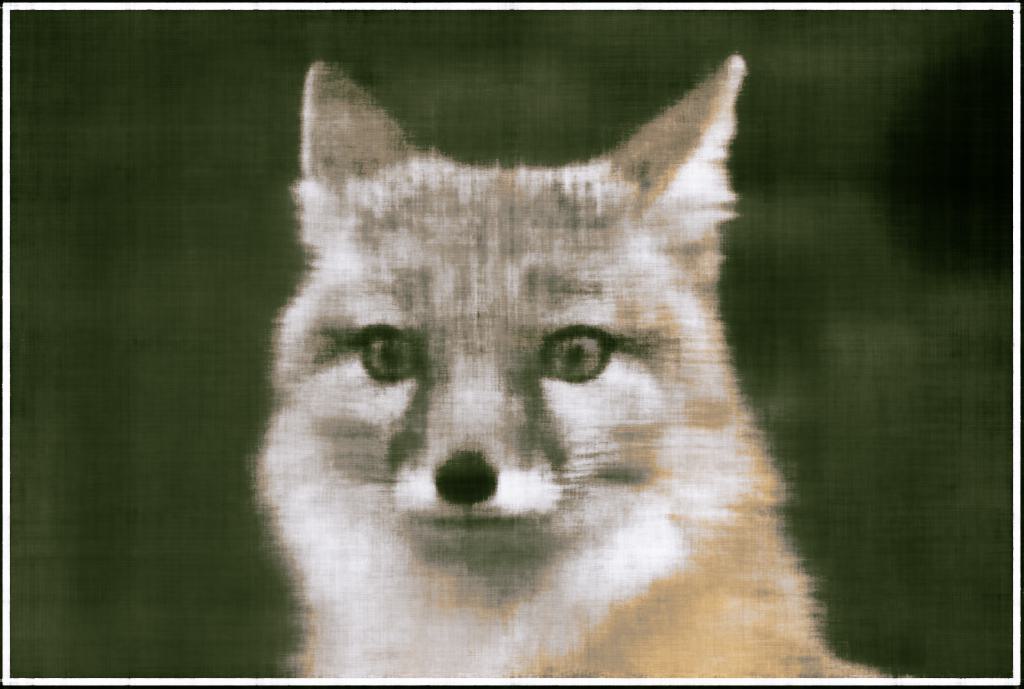
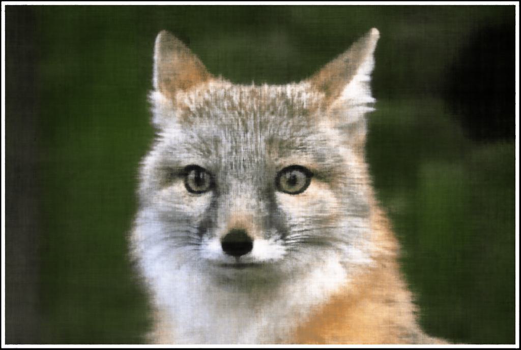
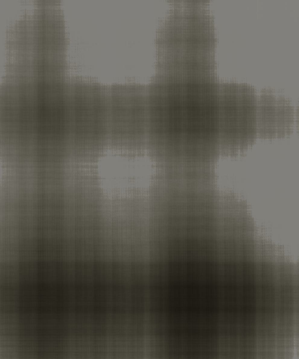
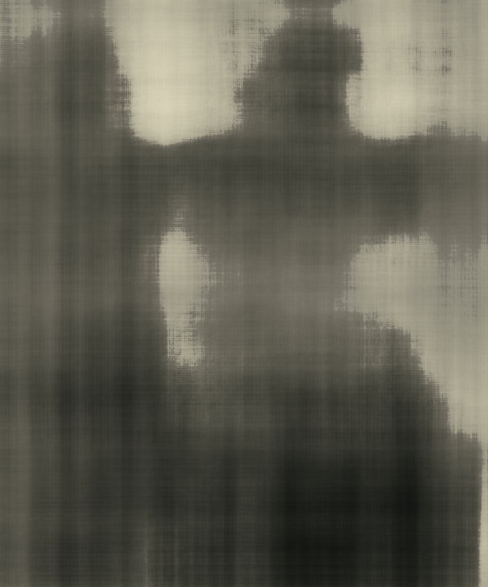
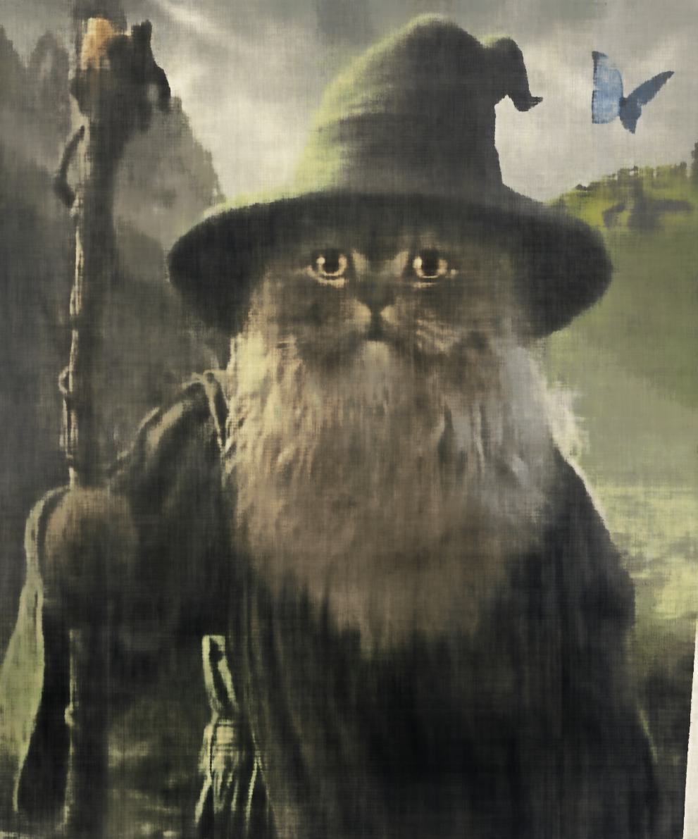
Here are the initial training results and intermediate reconstructions:

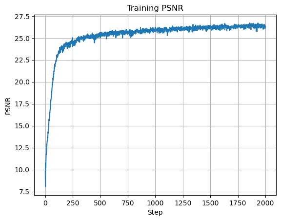
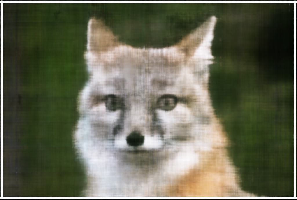
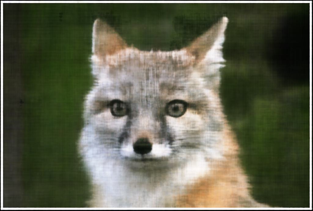
2D NeRF ground-truth fox image — Original image

2D NeRF final output — Final output, PSNR = 26.325

The model learns the underlying structure of the image and produces a reasonable reconstruction.

Hyperparameter Tuning

To better understand model behavior, I varied max frequency level, number of hidden layers, and number of hidden units.

Max Frequency Level

The max frequency level controls positional encoding dimensionality. Lower values can capture coarse structure, but high-frequency detail is lost without a large enough \(L\).

2D NeRF final output with L equals 1 — L = 1, PSNR = 23.366

2D NeRF final output with L equals 5 — L = 5, PSNR = 25.366

2D NeRF final output with L equals 10 — L = 10, PSNR = 26.325

Number of Hidden Layers

In an MLP, hidden layers are the fully connected layers between input and output. I varied this count from the original setup to evaluate reconstruction quality and convergence behavior.

2D NeRF final output with one hidden layer — 1 hidden layer, PSNR = 25.346

2D NeRF final output with two hidden layers — 2 hidden layers, PSNR = 26.325

2D NeRF final output with five hidden layers — 5 hidden layers, PSNR = 27.776

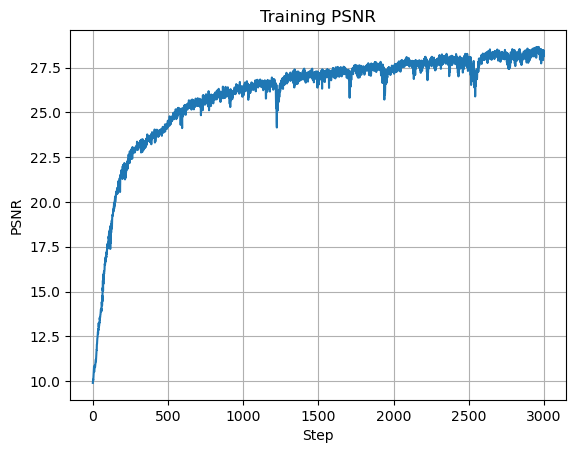
With deeper networks, training became harder, so I increased iterations and reduced learning rate. Best run here used \(10\) hidden layers, learning rate \(0.001\), and \(3000\) iterations for PSNR \(28.189\):

2D NeRF 10-layer model at iteration 50 — Iteration 50

2D NeRF 10-layer model at iteration 100 — Iteration 100

2D NeRF 10-layer model at iteration 200 — Iteration 200

2D NeRF 10-layer model at iteration 500 — Iteration 500

2D NeRF 10-layer model at iteration 1000 — Iteration 1000

2D NeRF 10-layer training PSNR curve — Training PSNR

2D NeRF 10-layer final output — Final output, PSNR = 28.189

Number of Hidden Units

The hidden-unit count controls layer width (model capacity). I tested several widths; larger models generally performed better but required more training to converge.

2D NeRF final output with 64 hidden units — 64 hidden units, PSNR = 24.8

2D NeRF final output with 128 hidden units — 128 hidden units, PSNR = 25.626

2D NeRF final output with 256 hidden units — 256 hidden units, PSNR = 26.325

2D NeRF final output with 400 hidden units — 400 hidden units, PSNR = 27.936

I used learning rate \(0.001\) and \(3000\) iterations for these larger models. The best run used \(512\) hidden units and reached PSNR \(27.696\):

2D NeRF 512-unit model at iteration 50 — Iteration 50

2D NeRF 512-unit model at iteration 100 — Iteration 100

2D NeRF 512-unit model at iteration 200 — Iteration 200

2D NeRF 512-unit model at iteration 500 — Iteration 500

2D NeRF 512-unit model at iteration 1000 — Iteration 1000

2D NeRF 512-unit training PSNR curve — Training PSNR

2D NeRF 512-unit final output — Final output, PSNR = 27.696

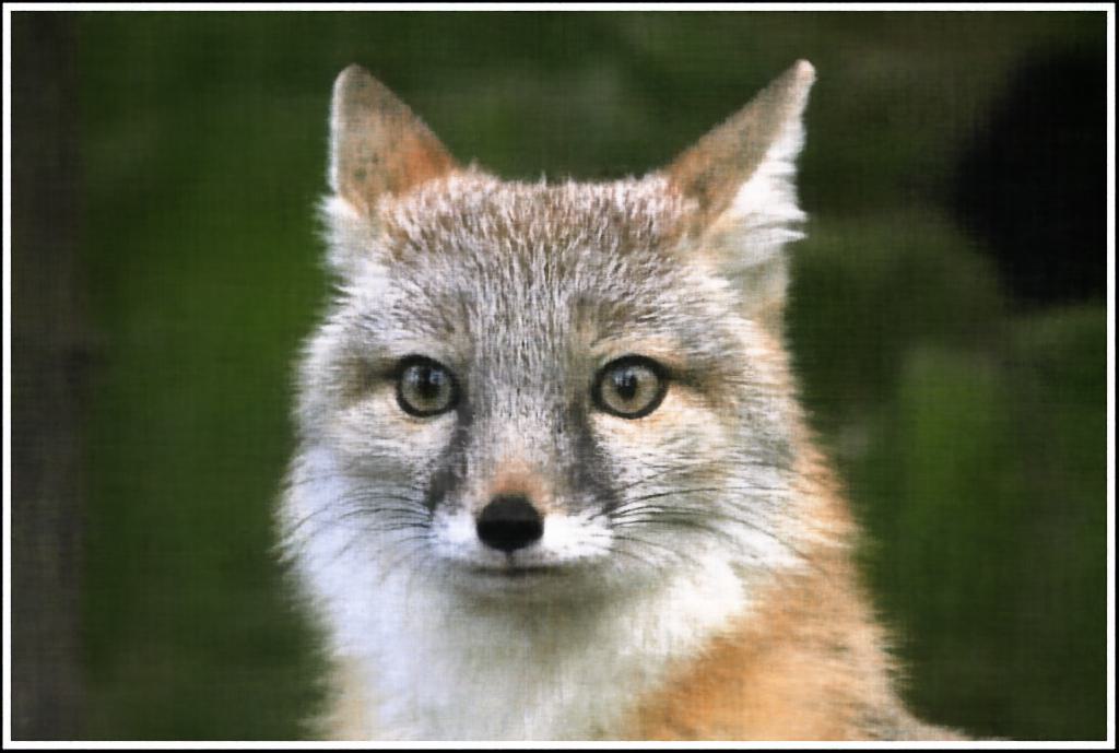
Conclusion

Increasing max frequency level, hidden layers, and hidden units all improved reconstruction quality, with clear compute and optimization trade-offs. For a stronger final 2D model, I chose \(L=10\), \(7\) hidden layers, \(512\) hidden units, learning rate \(0.001\), and \(3000\) iterations:

2D cat NeRF at iteration 0 — Iteration 0

2D cat NeRF at iteration 50 — Iteration 50

2D cat NeRF at iteration 100 — Iteration 100

2D cat NeRF at iteration 200 — Iteration 200

2D cat NeRF at iteration 500 — Iteration 500

2D cat NeRF at iteration 1000 — Iteration 1000

2D cat NeRF training PSNR curve — Training PSNR

2D cat NeRF final output — Final output, PSNR = 30.798

Part 2: Fitting a Neural Radiance Field from Multi-View Images

In the second part, I implemented the 3D NeRF model. The goal was to fit a radiance field to a 3D scene using multiple images and camera poses, then render novel views. I used the same dataset as the original NeRF paper, but at slightly lower resolution due to compute limits.

2.1 Creating Rays from Cameras

Camera-to-World Coordinate Conversion

The first step was implementing helper functions to define rays from camera parameters. We need to convert between camera-frame \(\mathbf{X}_c=(x_c,y_c,z_c)\) and world-frame \(\mathbf{X}_w=(x_w,y_w,z_w)\) coordinates:

\[ \begin{bmatrix} x_c \\ y_c \\ z_c \end{bmatrix} = \begin{bmatrix} \mathbf{R}_{3\times3} & \mathbf{t} \\ \mathbf{0}_{1\times3} & 1 \end{bmatrix} \begin{bmatrix} x_w \\ y_w \\ z_w \\ 1 \end{bmatrix} \]

The matrix above is the world-to-camera (w2c) transform (extrinsics). Its inverse is the camera-to-world (c2w) transform. I implemented transform(c2w, x_c) using NumPy and np.einsum for batched dimensions.

Pixel-to-Camera Coordinate Conversion

Next we map 2D pixels to camera coordinates using a pinhole camera model with focal lengths \(f_x, f_y\) and camera center \((o_x, o_y)\):

\[ \mathbf{K} = \begin{bmatrix} f_x & 0 & o_x \\ 0 & f_y & o_y \\ 0 & 0 & 1 \end{bmatrix} \]

Then:

\[ \begin{bmatrix} x_c \\ y_c \\ z_c \end{bmatrix} = \mathbf{K}^{-1} s \begin{bmatrix} u \\ v \\ 1 \end{bmatrix} \]

where \(s=z_c\) is depth along the optical axis. I implemented x_c = pixel_to_camera(K, uv, s) with batch support.

Pixel-to-Ray

Given camera coordinates, each ray has an origin and a direction.

\[ \mathbf{r}_o = -\mathbf{R}^{-1}_{3\times3}\mathbf{t}, \qquad \mathbf{r}_d = \frac{\mathbf{X}_w - \mathbf{r}_o}{\|\mathbf{X}_w - \mathbf{r}_o\|_2} \]

Using a point on the ray at depth 1 transformed to world space \(\mathbf{X}_w\), direction is:

\[ \mathbf{r}_d = \frac{\mathbf{X}_w - \mathbf{r}_o}{|\mathbf{X}_w - \mathbf{r}_o|_2} \]

I implemented ray_o, ray_d = pixel_to_ray(K, c2w, uv) with batched operation support.

2.2 Sampling

With rays defined, we sample 3D points along each ray. I typically used n_samples = 64 with near = 2.0 and far = 6.0 for the Lego scene. Points are sampled as \(\mathbf{x} = \mathbf{r}_o + \mathbf{r}_d t\). To reduce overfitting during training, I perturbed depths via t = t + (np.random.rand(t.shape)) * t_width with t_width = 0.02.

2.3 Dataloading

As in Part 1, we need a dataloader that returns random supervised samples. Here, it samples pixels from multi-view images, converts them to rays, and returns ray origins/directions plus target RGB values. I flattened pixels across all images and globally sampled \(N\) rays. I also accounted for pixel-center offset by adding 0.5 to the UV grid.

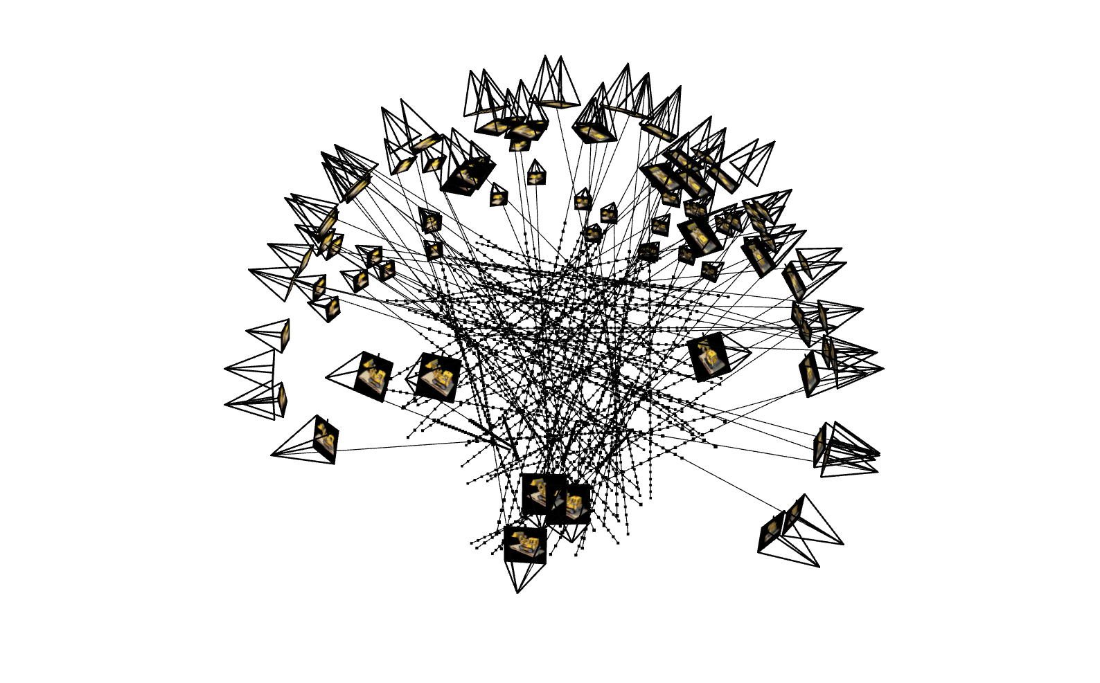
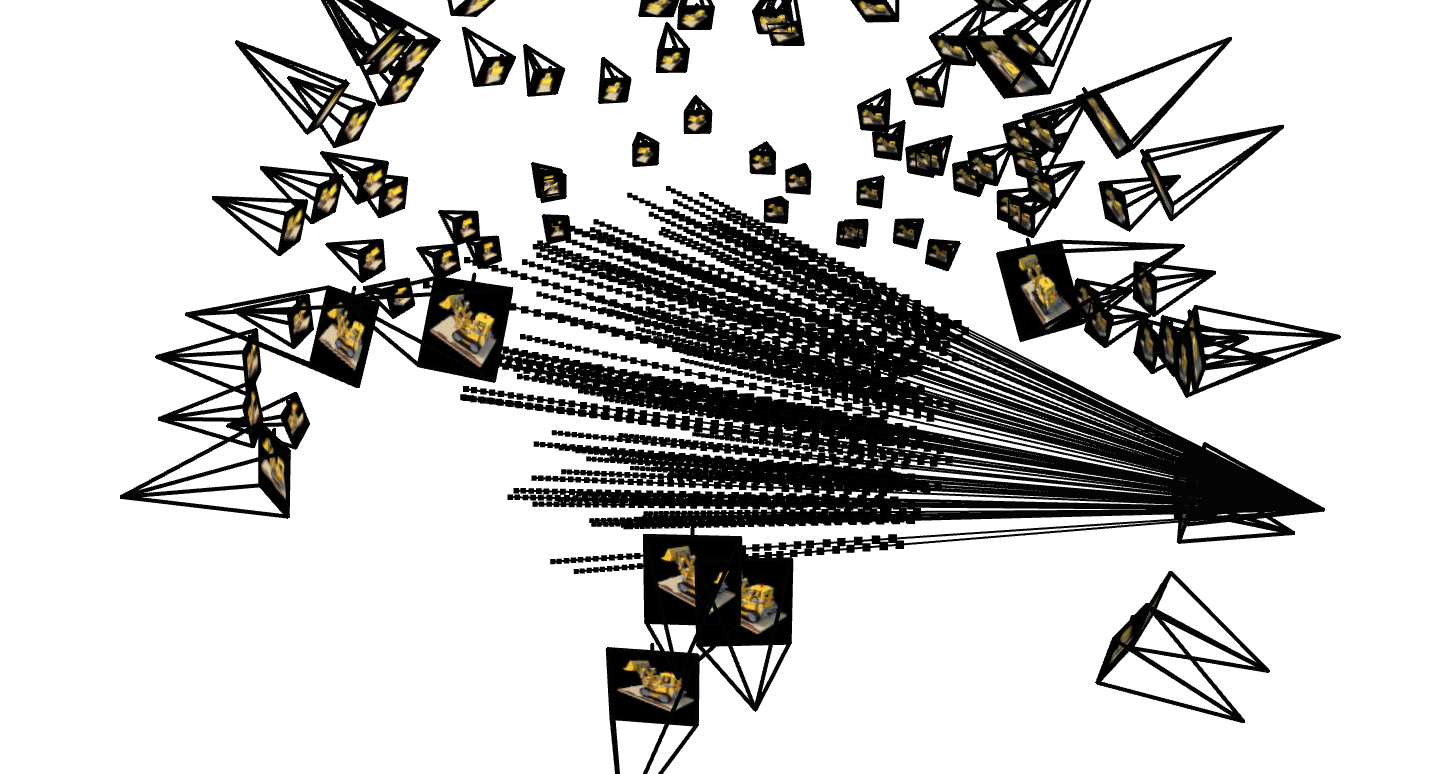
I verified correctness by visualizing sampled rays both across all views and from a single camera:

2.4 Neural Radiance Field

With data ready, I built the 3D NeRF network. This MLP takes both 3D position and view direction, and predicts RGB color plus density. I used positional encoding with \(L=10\) for position and \(L=4\) for direction.

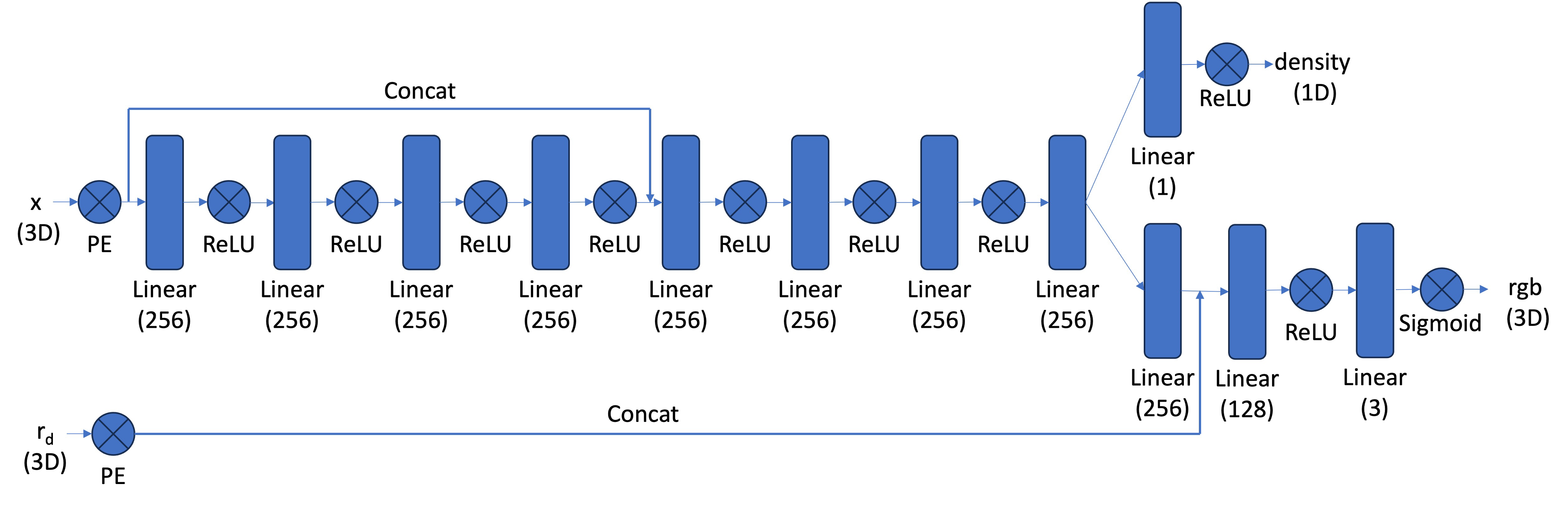
Because the model is deeper, I added a skip connection from input features to the middle layers to help preserve positional information. As in Part 1, output RGB is constrained to \([0,1]\) with Sigmoid activation.

2.5 Volume Rendering

The rendering step converts predicted densities and colors along a ray into one final pixel color:

\[ C(\mathbf{r}) = \int_{t_{near}}^{t_{far}} T(t)\sigma(\mathbf{r}(t))\mathbf{c}(\mathbf{r}(t), \mathbf{d})dt, \quad \text{where } T(t)=\exp\left(-\int_{t_{near}}^{t}\sigma(\mathbf{r}(s))ds\right) \]

In practice, we use a discrete approximation:

\[ \hat{C}(\mathbf{r}) = \sum_{i=1}^{N} T_i \alpha_i \mathbf{c}_i \]

where \(T_i\) is transmittance up to sample \(i\), and \(\alpha_i = 1 - e^{-\sigma_i \delta_i}\) is the probability of terminating at sample \(i\).

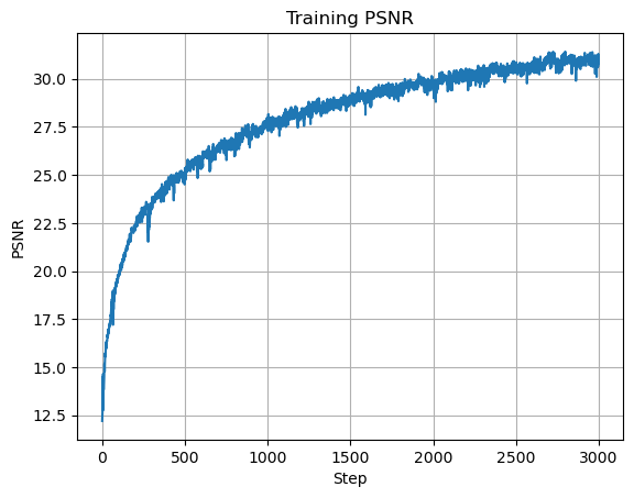
Training the Model

I trained with batch size \(10{,}000\), Adam optimizer, learning rate \(0.0005\), and \(3000\) iterations. This achieved final training PSNR \(26.062\) and validation PSNR \(24.96\).

3D NeRF at iteration 250 — Iteration 250

3D NeRF at iteration 500 — Iteration 500

3D NeRF at iteration 1000 — Iteration 1000

3D NeRF at iteration 2000 — Iteration 2000

NeRF training PSNR curve — Training PSNR

NeRF validation PSNR curve — Validation PSNR

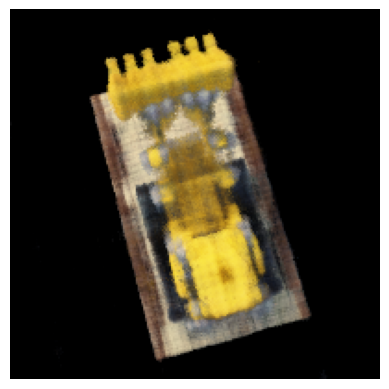
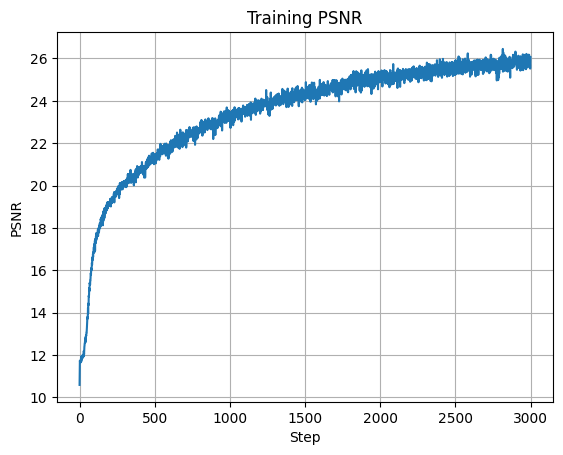
The model captures scene structure and enables novel-view synthesis:

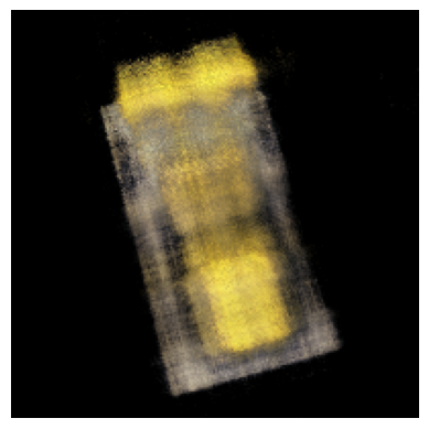
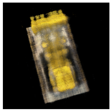
NeRF spherical rendering around Lego scene

Bells and Whistles

As an extension, I modified the rendering function to change the background color. Instead of only accumulating the probability of ray termination, I also used the probability that a ray never terminates and reaches the background. Multiplying that probability by a target background color produced alternate scene backgrounds: