Diffusion Models

In this project, we experimented with generating images using a diffusion model. A diffusion model is a generative model that is trained to iteratively remove the noise from an image. We can use this to generate images by starting with an image of pure noise and then applying the diffusion model to generate a new image on the manifold of "real" images. In part a, I explored the capabilities of diffusion models using a two-stage, pre-trained DeepFloyd IF model. In part b, I trained a diffusion model from scratch and tested it on images in the MNIST digits dataset.

Part 0: Playing with Diffusion

Note: To ensure deterministic outputs, for the rest of this part, I set the random seed \(180\).

In this part, we experimented with the DeepFloyd IF model, a pre-trained diffusion model that can generate images. This two-stage model was trained as a text-to-image model, and has 1000 timesteps in the diffusion process. We give this model some text embeddings that we can use to generate images. I used three prompts and tested out image generation using the DeepFloyd model, modifying the number of inference steps in the diffusion process for both stages of the model. Here are the resulting images and prompts I used:

" "

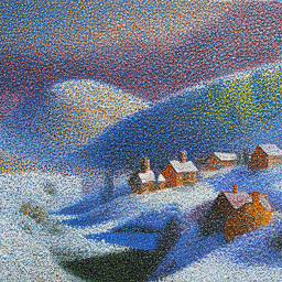
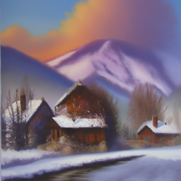
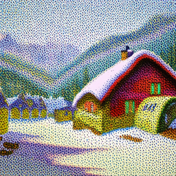
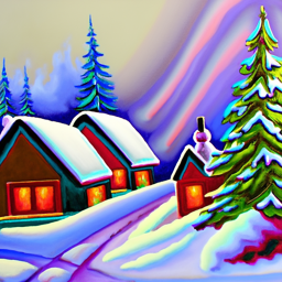
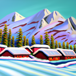
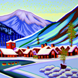
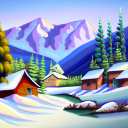
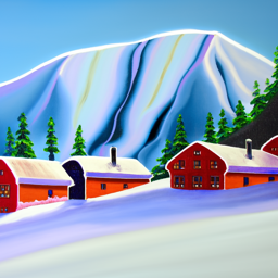
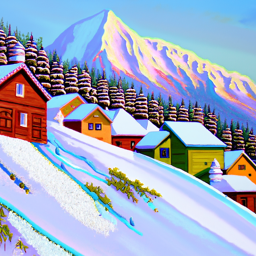
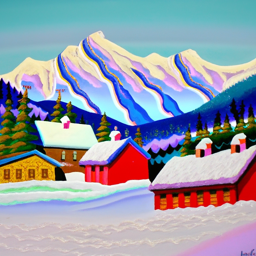
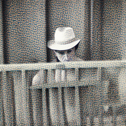
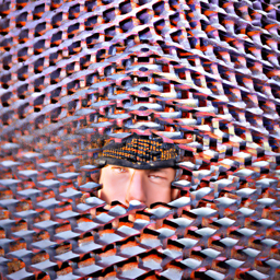
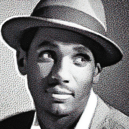
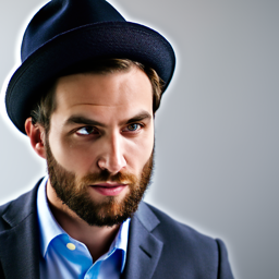
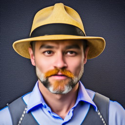
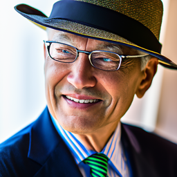
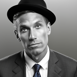
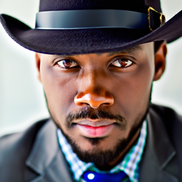
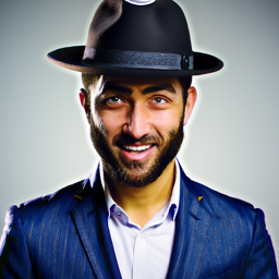
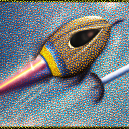
We can see that the number of steps in the diffusion process affects the quality of the generated images. With fewer steps, the images are more blurry and less detailed. With more steps, the images become more clear and detailed. The number of steps in the first stage of the diffusion process seems to affect the overall structure of the image, while the number of steps in the second stage affects the details. However, after a certain point, the image quality no longer seems to get any better.

Part 1: Sampling Loops

In this part we will be implementing sampling loops and using these loops to accomplish tasks such as inpainting and producing opticial illusions.

Forward Process:

We started this part by implementing the forward process of the diffusion model (noising and scaling an image), defined by the following equation: \[ q(x_t | x_0) = N\left(x_t; \sqrt{\bar{\alpha}}x_0, (1-\bar{\alpha}_t)\mathbf{I}\right) \] which is equivalent to: \[ x_t = \sqrt{\bar{\alpha}_t}x_0 + \sqrt{1 - \bar{\alpha}_t}\epsilon \quad \text{where} \quad \epsilon \sim N(0, \mathbf{I}) \] This gives us a noisy image \(x_t\) given a clean image \(x_0\). We not only add gaussian noise to our image, but also scale by our noise coefficients \(\bar{\alpha}_t\), coefficients that are close to \(1\) at the beginning of the diffusion process and close to \(0\) at the end. (Note: noise coeffiicents were chosen by the people who trained DeepFloyd). We can visualize our forward process on a small image of the Berkeley Campanile:

Classical Denoising:

We can now take these noisy images we genearted and try to remove the noise. One of the simplest methods we can use is to try a Gauussian blur filter to try to remove as much of the noise as possible. This is because noise is often quite high frequency, so blurring the image can help remove some of the noise.

Comparing to the noisy images above, it is clear that we have removed some noise, but the results still are not great. We still have very unclear images containing noise, especially for the images at higher timesteps.

One-Step Denoising:

We can try to do a better job of denoising by using our diffusion models (specifically within the first stage of our DeepFloyd model). This is a UNet that can be used to predict the Gaussian noise contained in the image. Once we have this noise, we can remove this noise and attempt to recover our original image. Since this is a test-to-image model, we also provide a text conditioning which is the prompt "a high quality photo."

Comparing to the Gaussian blur denoising, we can see that the one-step denoising does a much better job of removing the noise added to the image. We no longer see any of the small specs of noise in any of our images. However, we can still see that the results are quite blurry for higher tiemsteps.

Iterative Denoising:

In order to get our denoising to be even better, instead of jumping straight to the denoised image \(x_0\), we can attempt to take multiple steps to reach there. This can be done following this expression for a timestep \(t\) (where higher timestep means more noise): \[ x_{t'} = \frac{\sqrt{\bar{\alpha}_{t'}}\beta_t}{1-\bar{\alpha}_t}x_0 + \frac{\sqrt{\alpha_t}(1 - \bar{\alpha}_{t'})}{1-\bar{\alpha}_t}x_{t} + v_\sigma \] where

• \(x_{t}\) is the denoised image at timestep \(t\)
• \(x_{t'}\) is the denoised image at timestep \(t'\) where \(t'\lt t\) (less noisy)
• \(\bar{\alpha}_t\) is our denoising coefficients
• \(\alpha_t = \frac{\bar{\alpha}_t}{\bar{\alpha}_{t'}}\)
• \(\beta_t = 1-\alpha_t\)
• \(x_0\) is our current estimate of the clean image using the equation from the One-Step Denoising section
• \(v_\sigma\) is random noise predicted by our model

The intermediate steps can be thought of as a linear interpolation between the signal and noise. While we could go through all 1000 timesteps, we can also use a stride to speed up the process significantly without too much of a loss in quality. We chose a stride of 30 for our iterative denoising and started at timestep 990. We can then implement our iterative denoise:

We can see that the iterative denoising does a much better job of removing the noise from the image. The final image is much clearer and more detailed than the one-step denoising and Gaussian blur denoising. The iterative denoising process is able to remove the noise from the image while preserving most of the details of the original image.

Diffusion Model Sampling:

Now that we have an iterative denoise function, we can generate images from scratch. We can do so by starting from the first timestep and passing in purely random noise. We can then give it the prompt "a high quality photo" and run our iterative denoise function:

Classifier-Free Guidance (CFG):

We can see that our generated images are not particularly good, and some don't have any meaningful content in them. We can improve the quality of our images by using a technique called Classifier-Free Guidance (although this does sacrifice some image diversity). CFG is a technique where we use both a conditional noise estimate \(\epsilon_c\) and unconditional noise estimate \(\epsilon_u\) to form a new noise estimate. \[ \epsilon = \epsilon_u + \gamma(\epsilon_c - \epsilon_u) \] where \(\gamma\) is a hyperparameter that controls the strength of CFG. Our unconditioned noise estimate is given the empty string as a prompt and the conditioned noise estimate is once again given the prompt "a high quality photo."

We can see that the images generated with CFG are much better images than those generated by basic sampling. However, we can see that there is a loss in diversity in the images generated with CFG, as we have multiple images of landscapes at sunset. These are still a massive improvement in image quality, so we will use CFG in all of our image generation for the rest of this part.

Image-to-image Translation:

We can use a similar process as in our iterative denoising image to make edits to existing images. We can add noise to an image, and then denoise it to make edits to the image. The more noise we add, the greater the edits will be made. Intuitively, what this is doing is adding noise to an existing image, and then forcing it back onto the manifold of natural images. This is known as the SDEdit algorithm.

We can see that we are generating a range of images that gradually look more like the original as less noise is added.

Editing Hand-Drawn and Web Images

We can now do this same SDEdit procedure except by starting with nonrealistic images to start. We can experiment by using hand-drawn images and images taken from the web.

Inpainting

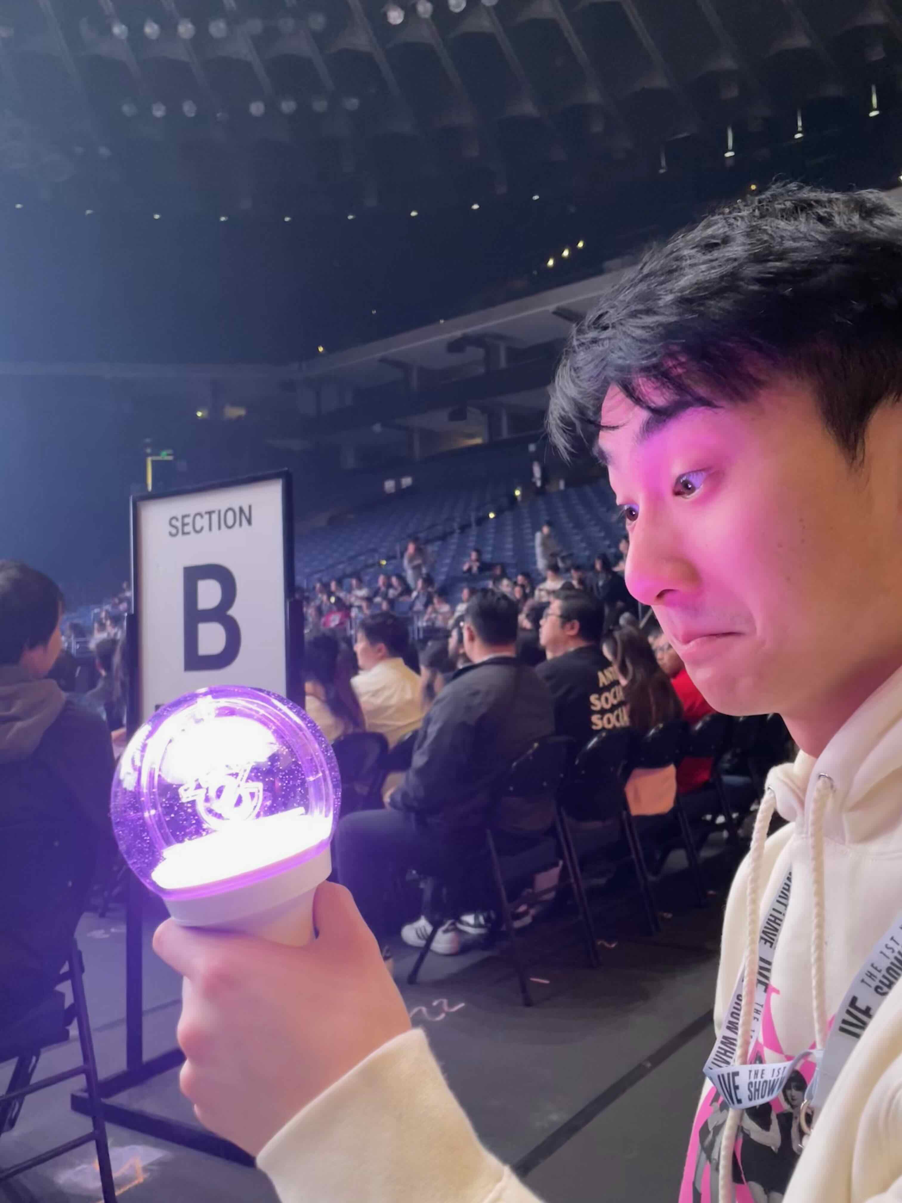
Another task we can accomplish with this process is inpainting. This is the same as the above portion except only for a chosen portion of our image. We can take in an original image \(x_{\text{orig}}\) and a binary mask \(\mathbf{m}\) that is 1 where we want to inpaint and 0 where we want to keep the original image. In our diffusion loop, our image is updated as follows: \[ x_{t} \leftarrow \mathbf{m}x_t + (1-\mathbf{m})\text{forward}(x_{\text{orig}}, t) \] This effectively replaces the masked portion of the image with the inpainted portion.

Text-Conditonal Image-to-image Translation

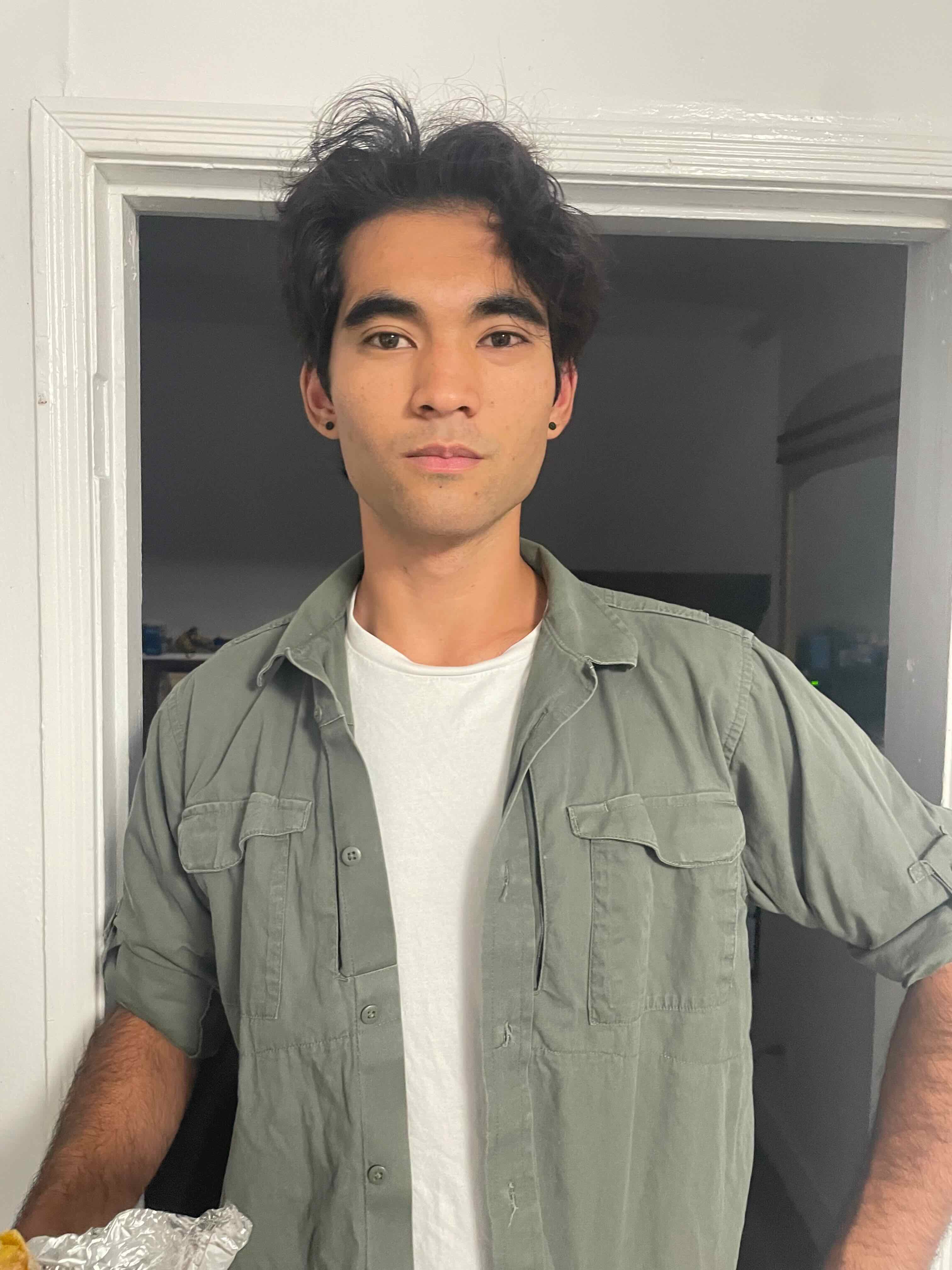
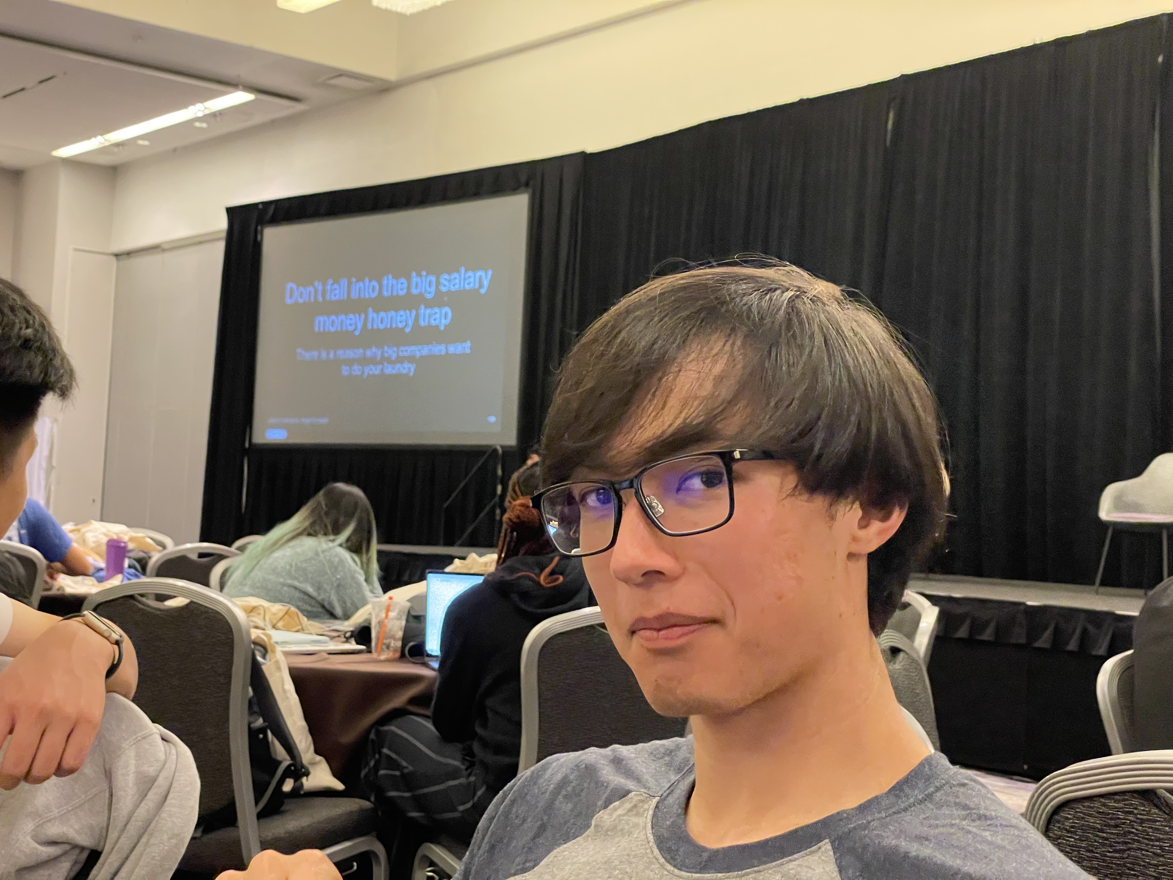
We can also guide the SDEdit process with a text prompt. We can do this simply by changing the text prompt from "a high quality photo" to a different text prompt of our choosing. Here are the results for different text prompts and images:

Visual Anagrams:

Another interesting task we can accomplish using the sampling loops we have defined is creating visual anagrams, where we see a different image when flipping the image over. We take the same steps of generating images based on text prompts by generating noise estimates for two images. However, after generating these images, we can average the noise estimates after flipping one of them before denoising to generate our anagram. Here is the algorithm: \begin{align*} \epsilon_1 &= \text{UNet}(x_t, t, p_1) \\ \epsilon_2 &= \text{flip}(\text{UNet}(x_t, t, p_2)) \\ \epsilon &= \frac{\epsilon_1 + \epsilon_2}{2} \end{align*} where \(p_1\) and \(p_2\) are the text prompts for the two images, and flip() is a function that rotates the images 180 degrees. Once we have this new noise estimate we can implement the same denoising process to arrive at our anagrams.

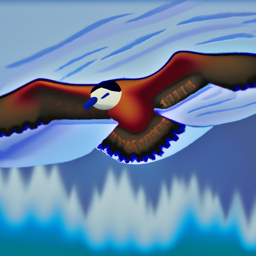
Hybrid Images

One final task we can accomplish with our diffusion model sampling loops is forming hybrid images, images that show the one image close up, and a different image from far away. We can do this in a similar way to the anagrams, where we generate noise estimates for two images, but instead of averaging them, we can sum the low frequency images from one image and high frequency components of another image. Here is the algorithm: \begin{align*} \epsilon_1 &= \text{UNet}(x_t, t, p_1)\\ \epsilon_2 &= \text{UNet}(x_t, t, p_2)\\ \epsilon &= f_{LP}(\epsilon_1) + f_{HP}(\epsilon_2)\\ \end{align*} We use a gaussian blur of kernel size 33 and sigma 2 for our lowpass filter, and a highpass filter is defined as the original noise minus the lowpass noise obtained by the gaussian filter. Once we have this new noise estimate we can implement the same denoising process to arrive at our hybrid images:

Part B: Diffusion Models from Scratch!

In this project, we implemented our own diffusion models from scratch using PyTorch. We trained our model on the MNIST numbers dataset.

Part 1: Training a Single-Step Denoising UNet

We first trained a simple one-step denoiser that takes in a noisy image and outputs a denoised image by optimizing the L2 loss: \[ L = \mathbb{E}_{z, x}||D_\theta(z) - x||^2 \]

Implementing the UNet

We implemented a simple UNet architecture with some downsampling blocks, upsampling blocks, and skip connections. We started by defining a bunch of simple operation blocks such as Convolution blocks, Downsampling blocks, flattening blocks, and concatenation blocks. Here is our overall system architecture:

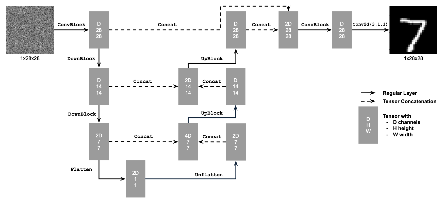
Using the UNet to Train a Denoiser

We trained our UNet architecture using the MNIST dataset. We generated training data pairs of \((z, x)\) where \(x\) is a clean MNIST digit and we generated \(z\) by adding noise to \(x\): \[ z = x + \sigma \epsilon \quad \text{where} \epsilon \sim \mathcal{N}(0, 1) \] This gives us noisy images we can train our UNet to denoise using the L2 loss function defined above.

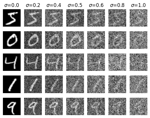
Training

We trained our model for 5 epochs on the torchvision.datasets.MNIST dataset, shuffling the data using a dataloader. We generated our noisy images using a value of \(\sigma = 0.5\) and a hidden dimension of 128. We trained in batches of size 256 using the Adam Optimizer and a learnring rate of 1e-4.

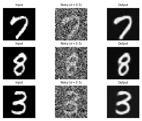
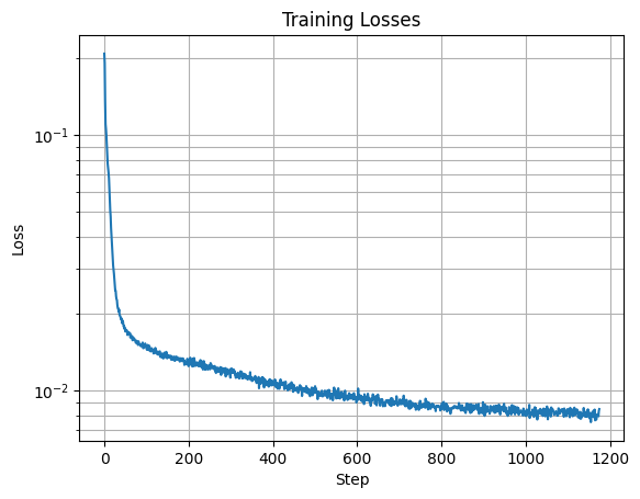
Here are the results of our training:

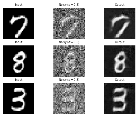
Out-of-Distribution Testing

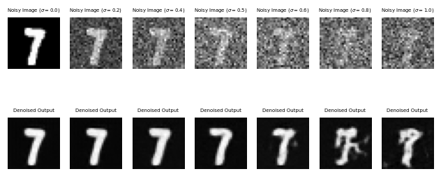
While we trained our UNet on denoising images noised with \(\sigma=0.5\), we can test our model on images noised with other values of \(\sigma\). We can visualize our results on images noised with varying levels of noise: \[ \sigma = [0.0, 0.2, 0.4, 0.5, 0.6, 0.8, 1.0] \]

Part 2: Training a Diffusion Model

Now we can train an iterative denoising UNet model based on the DDPM model. Now instead of using our UNet to predict the clean image, we are now training our UNet to predict the noise that was added to the image. This means our UNet will now use the following loss function: \[ L = \mathbb{E}_{\epsilon, z}||\epsilon_\theta(z) - \epsilon||^2 \] where \(\epsilon_\theta\) is the UNet model trained to predict noise.

We also must define our timestep noise coefficients \(\bar{\alpha}_t\), which we do based on the lists \(\alpha\) and \(\beta\).

• \(\beta\) (variance scheduler): \(\beta_0 = 0.0001\) and \(\beta_T = 0.02\) and all other elements \(\beta_t\) for \(t \in \{1, \dots, T-1\}\) are evenly spaced between the two
• \(\alpha_t = 1 - \beta_t\)
• \(\bar{\alpha}_t = \prod_{s=1}^{t} \alpha_s\) is a cumulative product of \(\alpha_s\) for \(s \in\{1, \dots, t\}\)

Since we are dealing with simpler images in the MNIST dataset, we can use a smaller number of timesteps \(T=300\). We can then train our model with the time conditioned loss function: \[ L = \mathbb{E}_{\epsilon, x_0, t} ||\epsilon_\theta(x_t, t) - \epsilon||^2 \]

Adding Time Conditioning to UNet

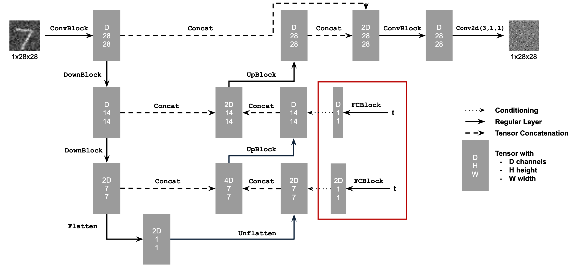
We need to inject our scalar value \(t\) into our model in order to condition on it. One way we can accomplish this is to add the scalar value as an input to a Fully-Connected block which then adds the time conditioning into the model before both Upsampling Blocks. We also normalize our \(t\) values to between 0 and 1 before inputting it into our model.

Training the UNet

We train our time-conditioned UNet by repeatedly picking a random image from our training set, picking a random t, and training our denoiser to predict the nosie in \(x_t\) until it converges.

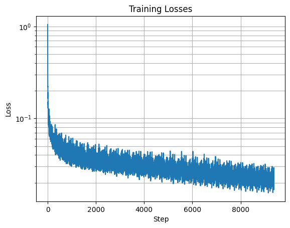
We once again used the MNIST dataset and shuffled the data using a dataloader. This time, we used a batch size of 128 and trained our model for 20 epochs due to the increased difficulty of this task. We used a hidden dimension of 64 and trained using the Adam optimizer with an initial learning rate of 1e-3. We also used an exponential decay learning rate scheduler with gamma of \(0.1^{(1.0/\text{num_epochs})}\), updating our step after every epoch.

Sampling from the UNet

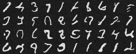
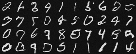
We can now sample from our trained UNet to generate images, and is similar to our sampling process from part A. We can generate a random noise vector \(z\) and then iteratively denoise it using our trained UNet and the timestep noise coefficients we defined above.

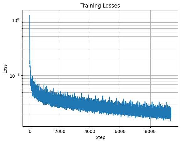
Here are the results of our training and sampling process:

Adding Class-Conditioning to UNet

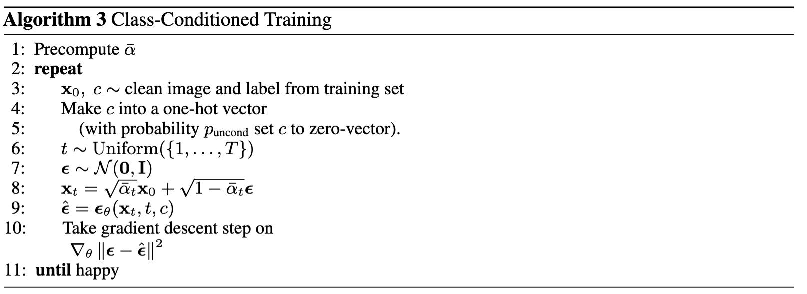
To further improve our results, we can add class-conditioning to our UNet architecture. We can do so by conditioning our model using the labels of our MNIST dataset. We can add a one-hot encoded vector \(c\) to our model that represents the class of the image we are trying to denoise. We still want our UNet to be able to work without conditioning, so we also implement a dropout 10% of the time by setting our vector \(c\) to 0.

We implement our class-conditioning using the same process as our time-conditioning. We add two more Fully-Connected Blocks into our model and multiply the blocks before each Upsample by the class-conditioning, as well as adding the time-conditioning blocks.

Sampling from the Class-Conditioned UNet

From part a, we know that simple conditional sampling does not produce great results. Therefore, in our sampling process we once again use classifier-free guidance along with our class conditioning.

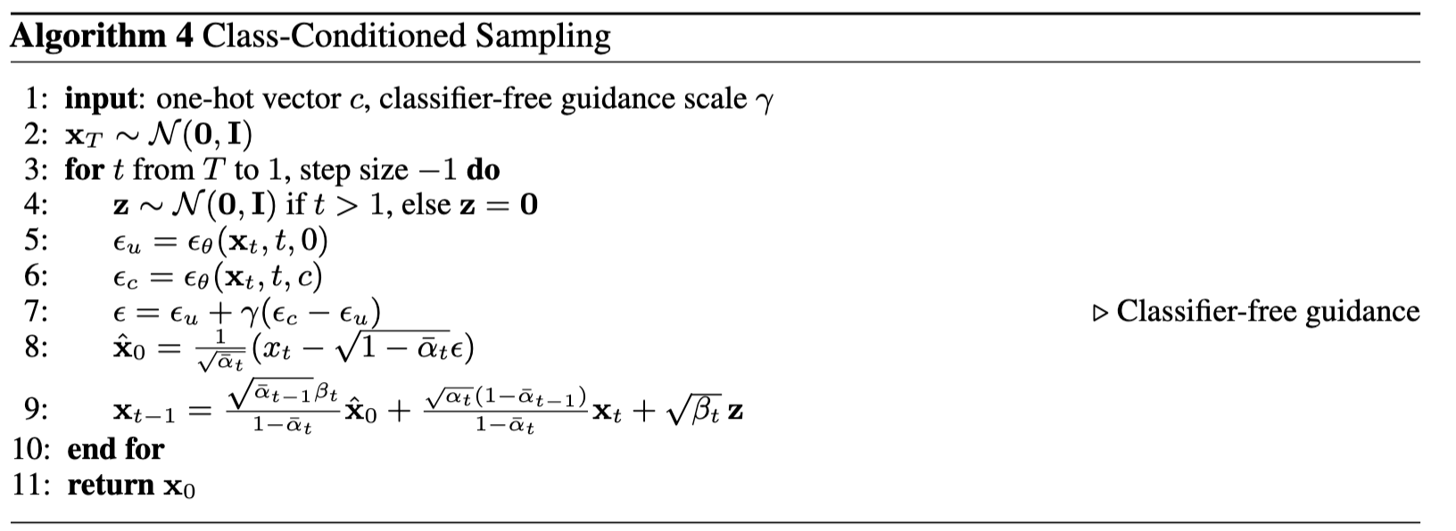
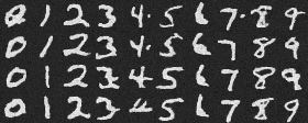
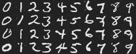
Here are the final results of our class-conditioned UNet

Conclusions

This project of messing with diffusion models was quite interesting. I enjoyed being able to play around with the DeepFloyd model and see the results of the different tasks we could accomplish with it. I found the picture anagrams to be particularly interesting, since this created some very interesting images. I also found getting to implement our own simple UNet and Diffusino models to be a good and informative experience. I think this process really helped me learn more about diffusion models and how they can be used to accomplish a variety of tasks.