Fun with Filters and Frequencies

By: Evan Chang

CS 180 Project 2

Part 1: Fun with Filters

Finite Difference Operator

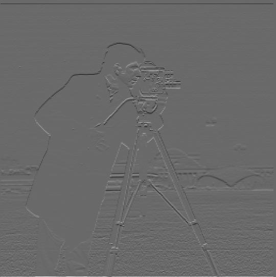
A common task in image processing is finding the edges in an image along both the horizontal and vertical directions. This is often done by computing the gradients of the image along the x and y directions. This can be simply done by convolving the image with simple kernels that approximate the derivative of the image using finite differences. These kernels are simply taking the difference between two consecutive pixels in the image as an approximation of the true derivative. $$\text{Gradient in x direction: } \matrix{D_x} = \begin{bmatrix} 1 -1 \end{bmatrix}$$ $$\text{Gradient in y direction: } \matrix{D_y} = \begin{bmatrix} 1 \\ -1 \end{bmatrix}$$
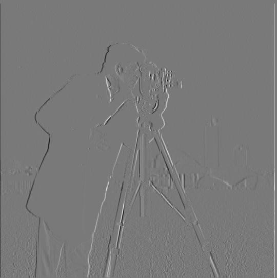
Image Gradient (dx)
Image Gradient (dx)
Image Gradient (dy)
Image Gradient (dy)
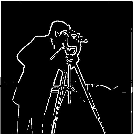
We can also compute the magnitude of the gradient by taking the square root of the sum of the squares of the gradients in the x and y directions to visualize the edges in the image. In order to remove some of the noise, we also can threshold the gradient magnitude to get a clearer picture of the edges in the image.
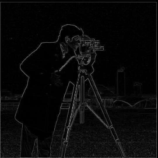
Image Gradient Magnitude
Thresholded Image Gradient Magnitude
Thresholded Image Gradient Magnitude (threshold=0.27)

Derivative of Gaussian (DoG) Filter

We can also smooth out our gradient magnitude edges by smoothing image first using a Gaussian filter. Convolving our image with a Gaussian filter gives us a cleaner picture of the edges. When we thresholded, we could tell we were only displaying the stronger edges and there was less noise in the image. However, there were also some gaps in the edges that we did have due to this thresholding. We can see in the smoothed version that the edges are more continuous and there are less gaps in the edges.
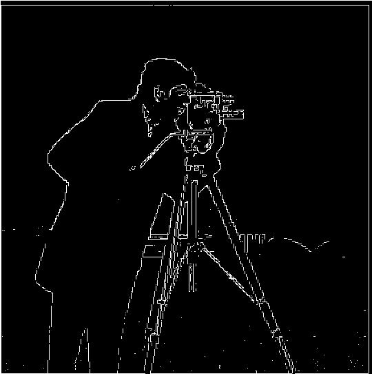
Thresholded Image Gradient Magnitude
Thresholded Image Gradient Magnitude (non-smoothed)
Thresholded Image Gradient Magnitude (smoothed)
Due to the linear nature of convolutions, we can also compute this smoothed gradient magnitude using only one filter instead of two. This filter is known as the Derivative of Gaussian (DoG) filter and works by convolving the Gaussian with the finite difference operators first. Since these are much smaller than the image, we can convolve the Gaussian with the finite difference operators first and then convolve the result with the image to get the same result in less time.
Image Gradient with Two Convolutions
Two Convolutions
Image Gradient (DoG)
Single Convolution (DoG filter)
Part 2: Fun with Frequencies!

Image Sharpening

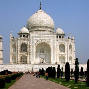
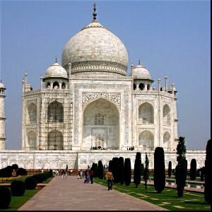
Another common task in image processing is image sharpening. A simple way we can accomplish this is by simply adding more of the high frequency components back into the image. We can get the high frequency portions by simply subtracting the blurred image from the original image. This will give us the high frequency components of the image which we can add back with an enhancement factor to "sharpen" the image. Combining these operations into one filter gives us the unsharp mask filter. The process is outlined below for two example images:
Image Sharpening Process
Costco Sharpening Process
Here are some results from testing this filter on several blurry images.
Sharpened Image
Original Image
Original Image
Sharpened Image
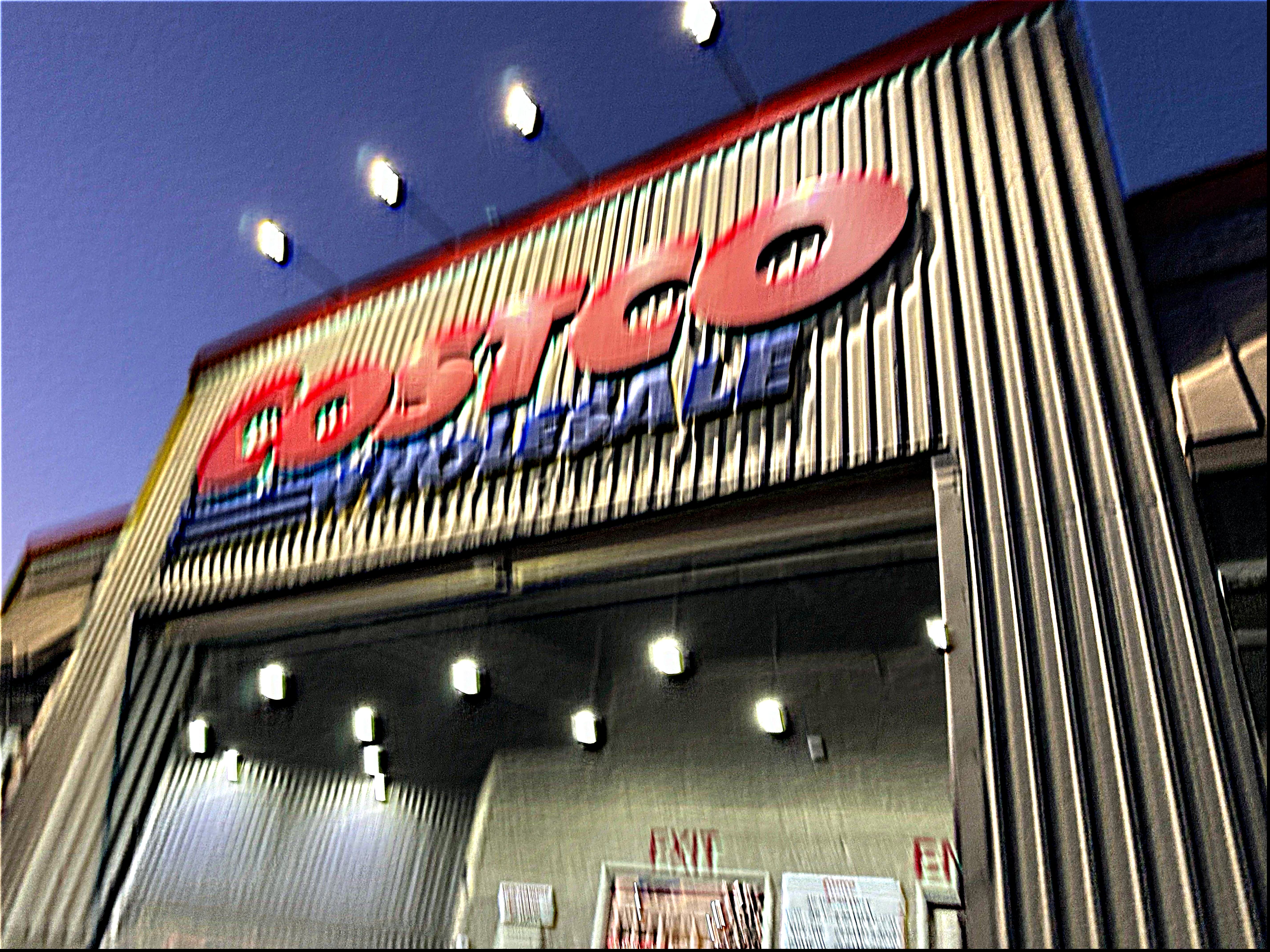
Picture of Blurry Costco's Entrance
Blurry Costco
Sharpened Costco
Sharpened Costco
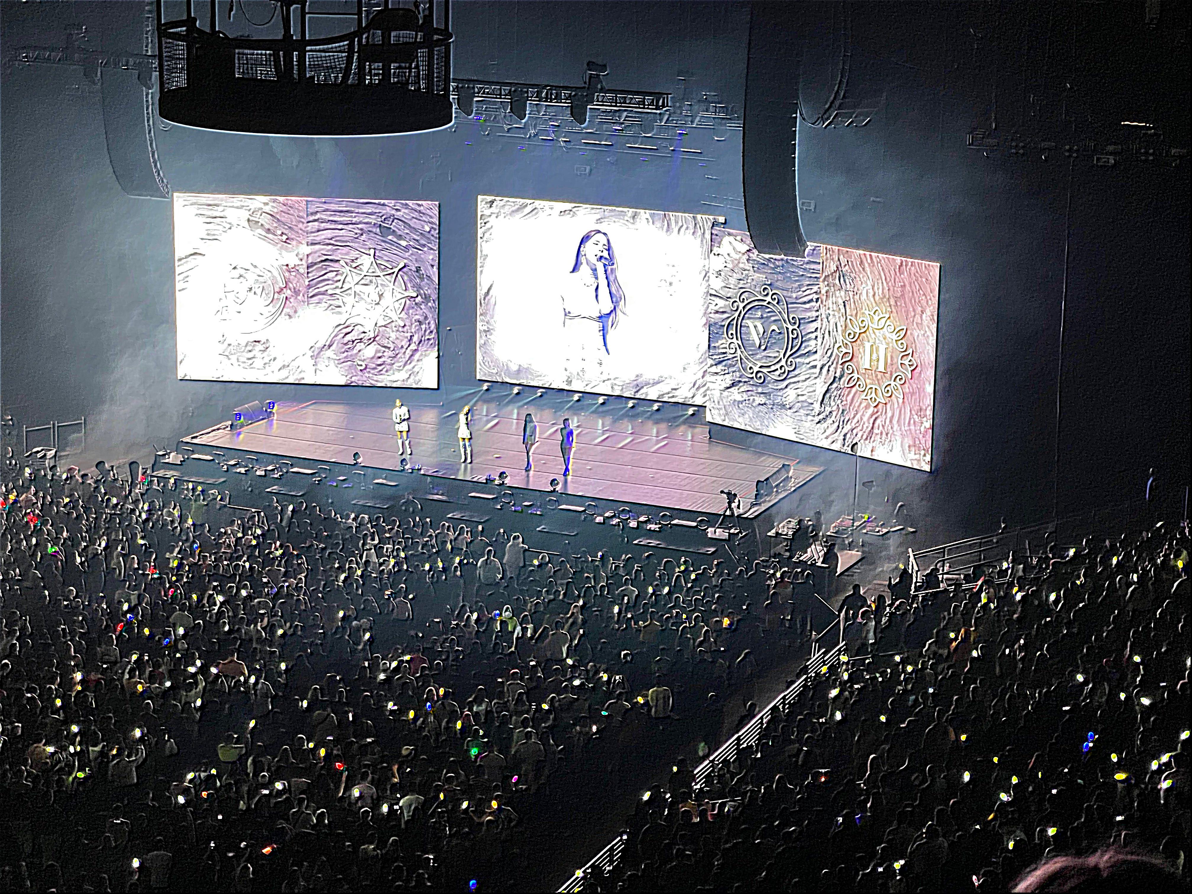
Blurry Picture of Concert Stage
Blurry Concert Image
Sharpened Concert
Sharpened Concert Image
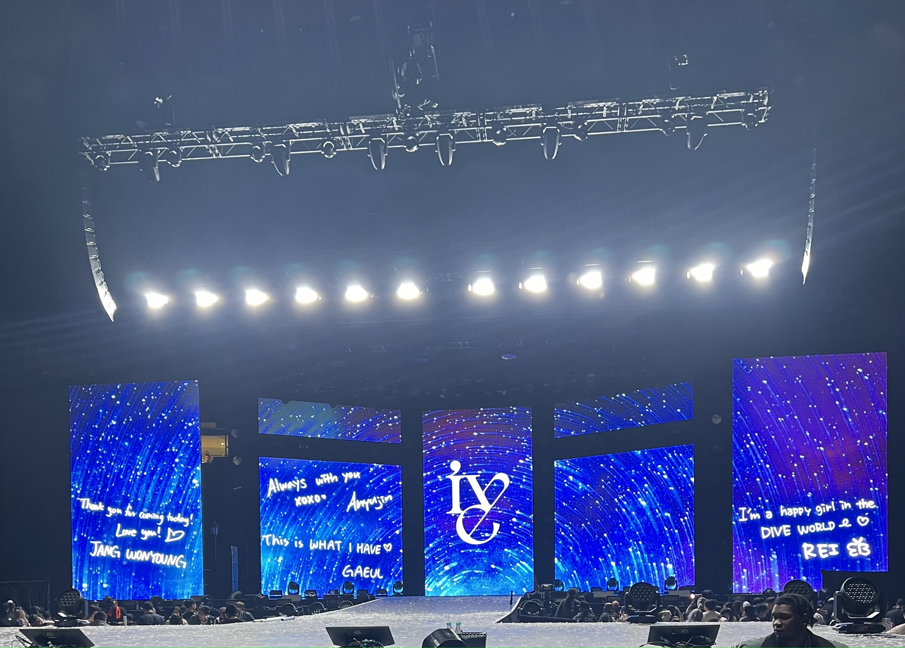
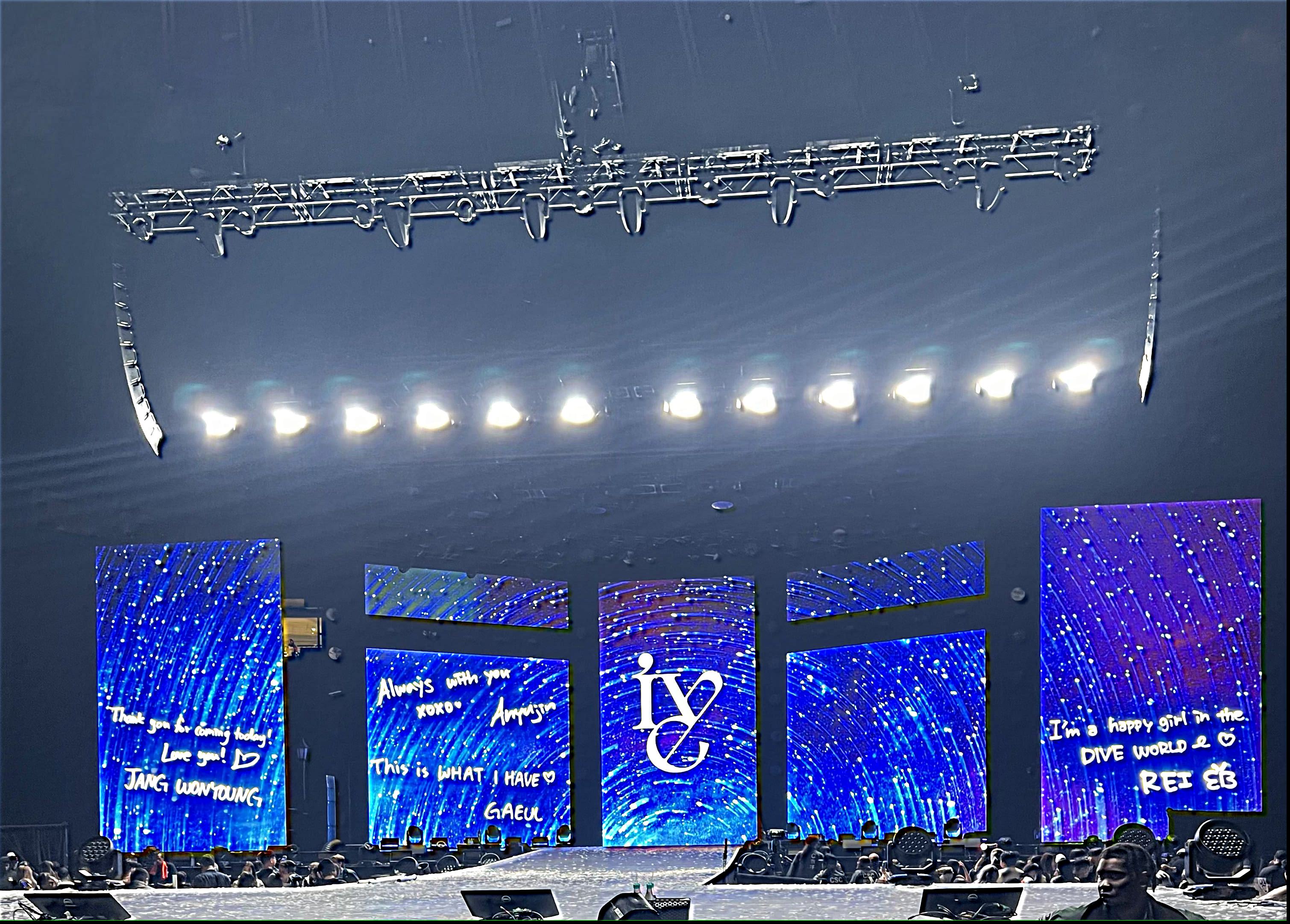
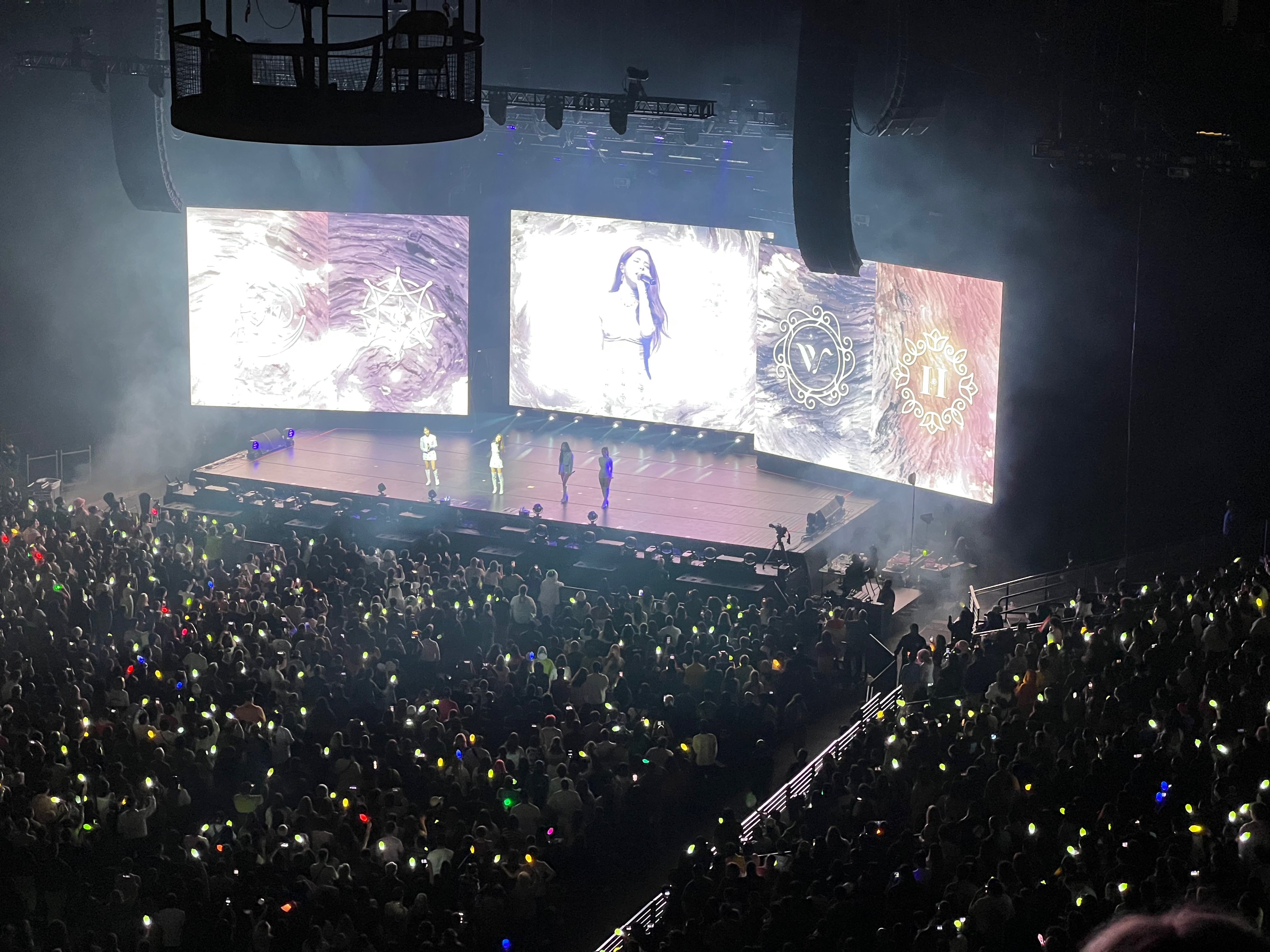
Blurry Picture of IVE concert
Blurry IVE Concert Image
Sharpened IVE Concert
Sharpened IVE Concert Image
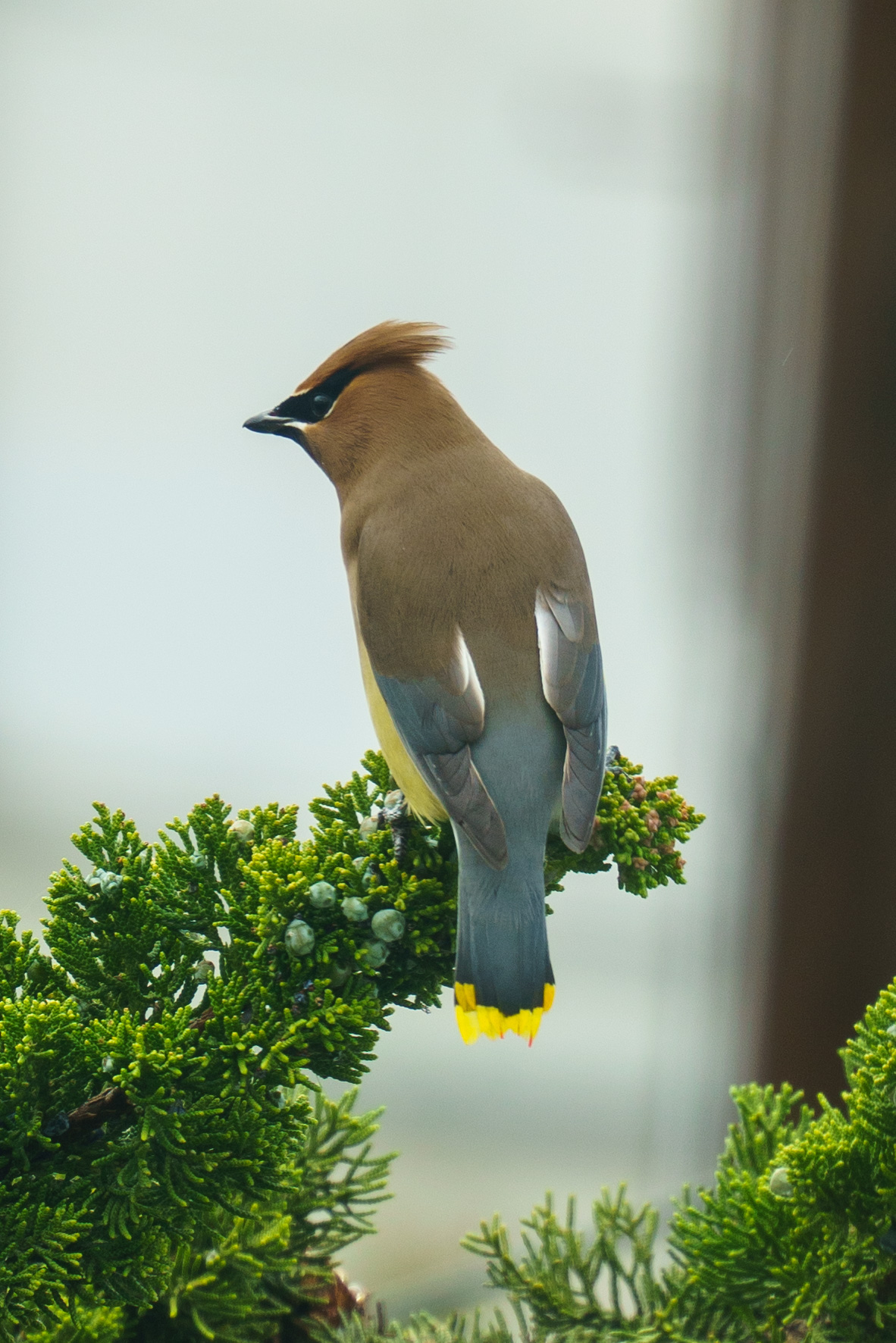
Picture of Cedar Waxwing in a tree
(Not so Blurry) Bird Picture
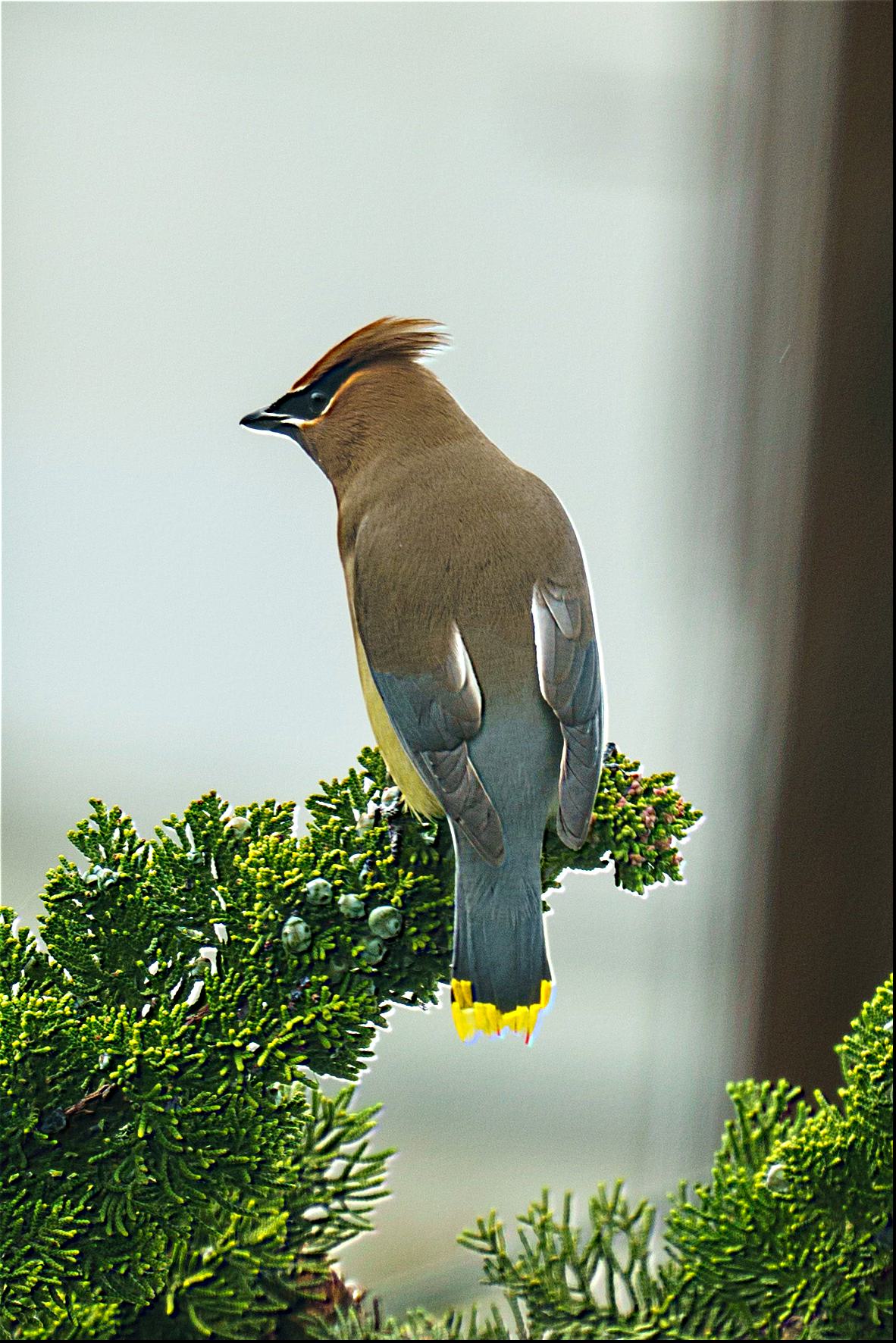
Sharpened picture of Cedar Waxwing in a tree
Sharpened Bird Picture
From these examples, we can see that the unsharp mask filter does a good job of enhancing some of the higher frequency components. It does particularly good with the lines in building structures. However, it is far from perfect as an unblurring filter since it is only able to enhance the edges that are already present in the image. It is not able to recover any lost details from the original image. For fun, this is what happens when we apply the unsharp mask filter to a blurred and re-sharpened image:
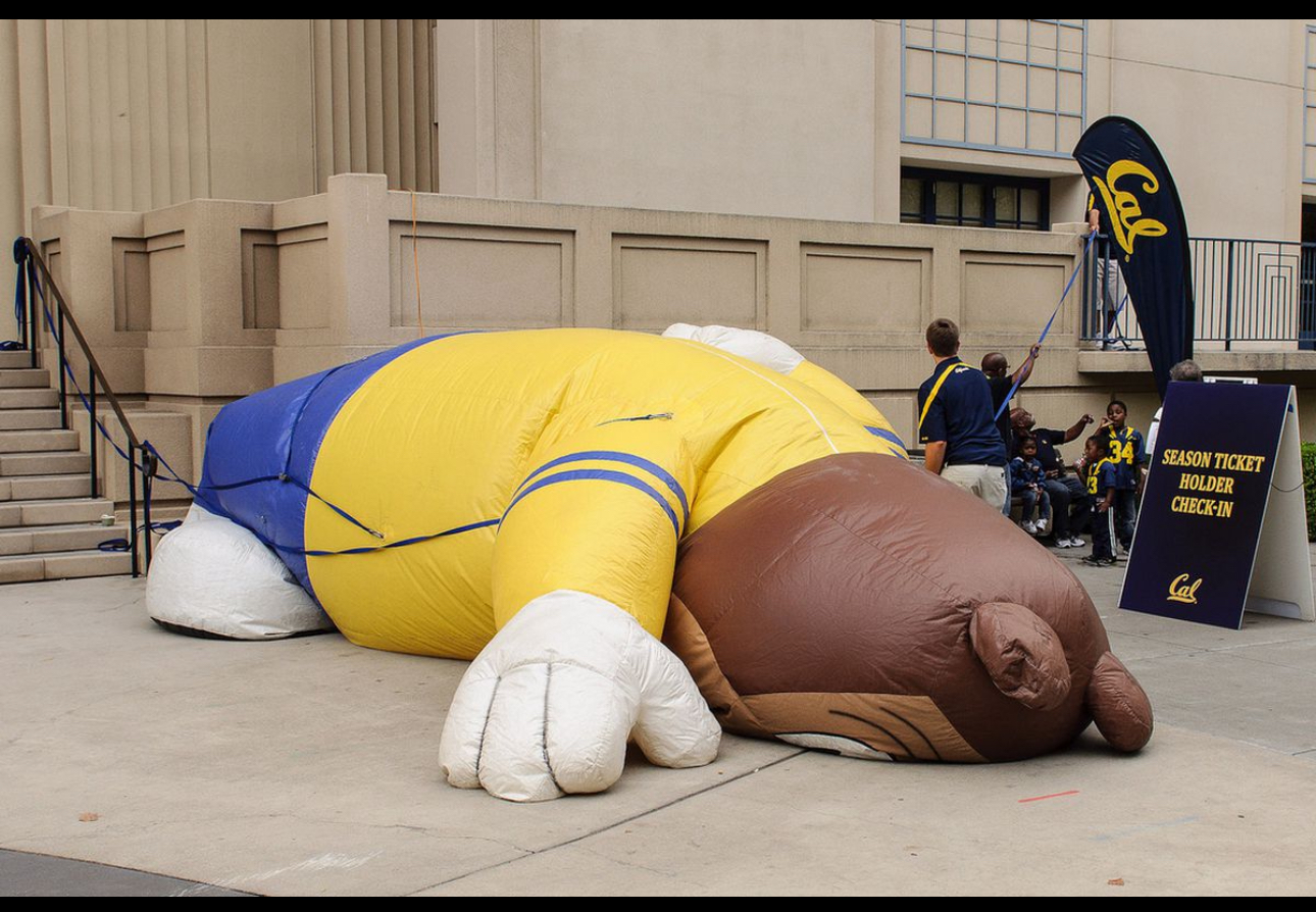
Picture of Oski
Oski
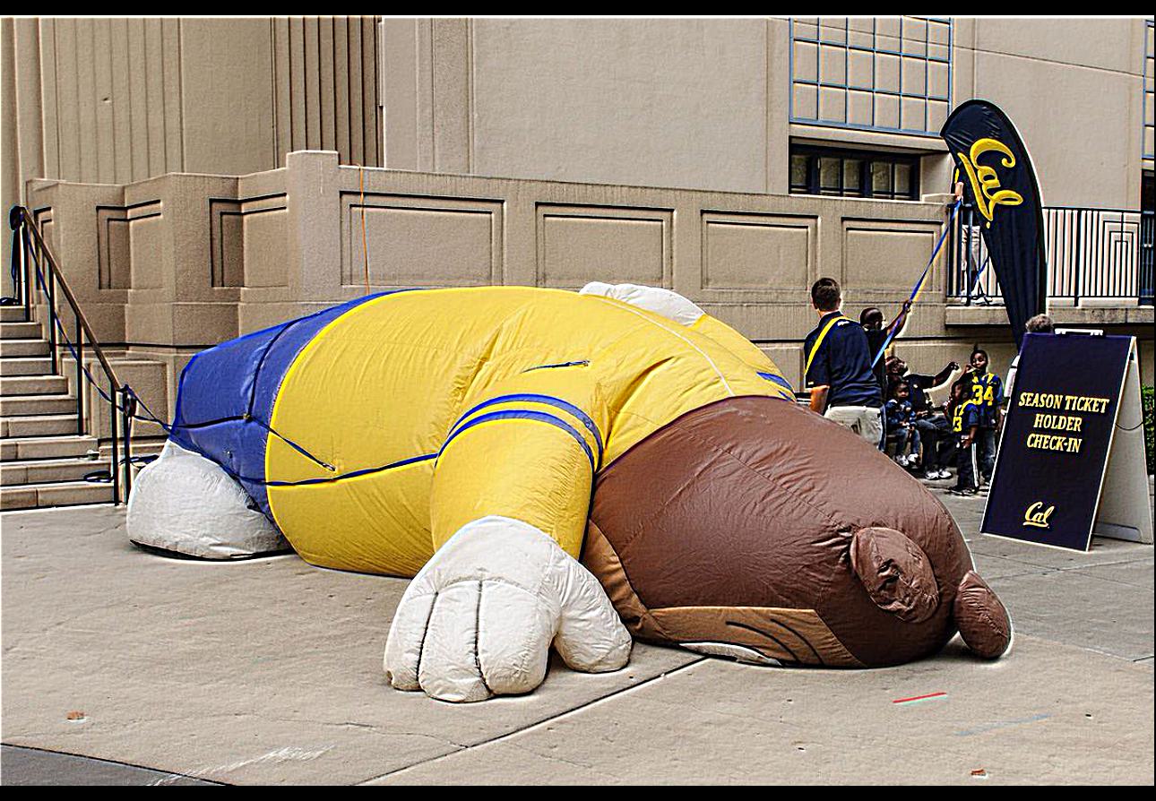
Sharpened Oski
Sharpened Oski
This image was already decently sharp. I then attempted to blur it and re-sharpen it. The result is an image of oski with even sharper edges than the original.

Hybrid Images

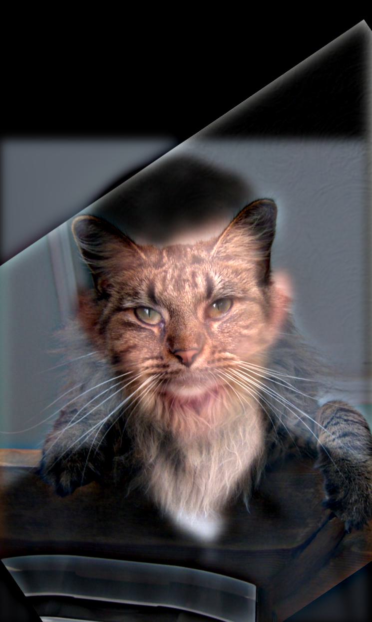
In this section, we will be creating hybrid images by combining the low frequency components of one image with the high frequency components of another image. Since human's perceive low frequency much better than high frequency, up close, we will see mostly the image with low-pass components. However, when viewed from afar, we can see the elements of the high-pass filtered image. Similar to before, we can get the low-pass components by blurring the image with a Gaussian filter. We can get the high-pass components by subtracting the low-pass filtered image from the original image. We then can average the two filtered images to produce our hybrid image. We can control the amount of high frequency components in the image by adjusting the sigma of the Gaussian filter. The higher the sigma, the more high frequency components we will have in the image. This is also the same for the low frequency components. Before doing this, in order for the image to hybridize properly, we first aligned the two images by matching up two points and resizing them to the same dimensions.
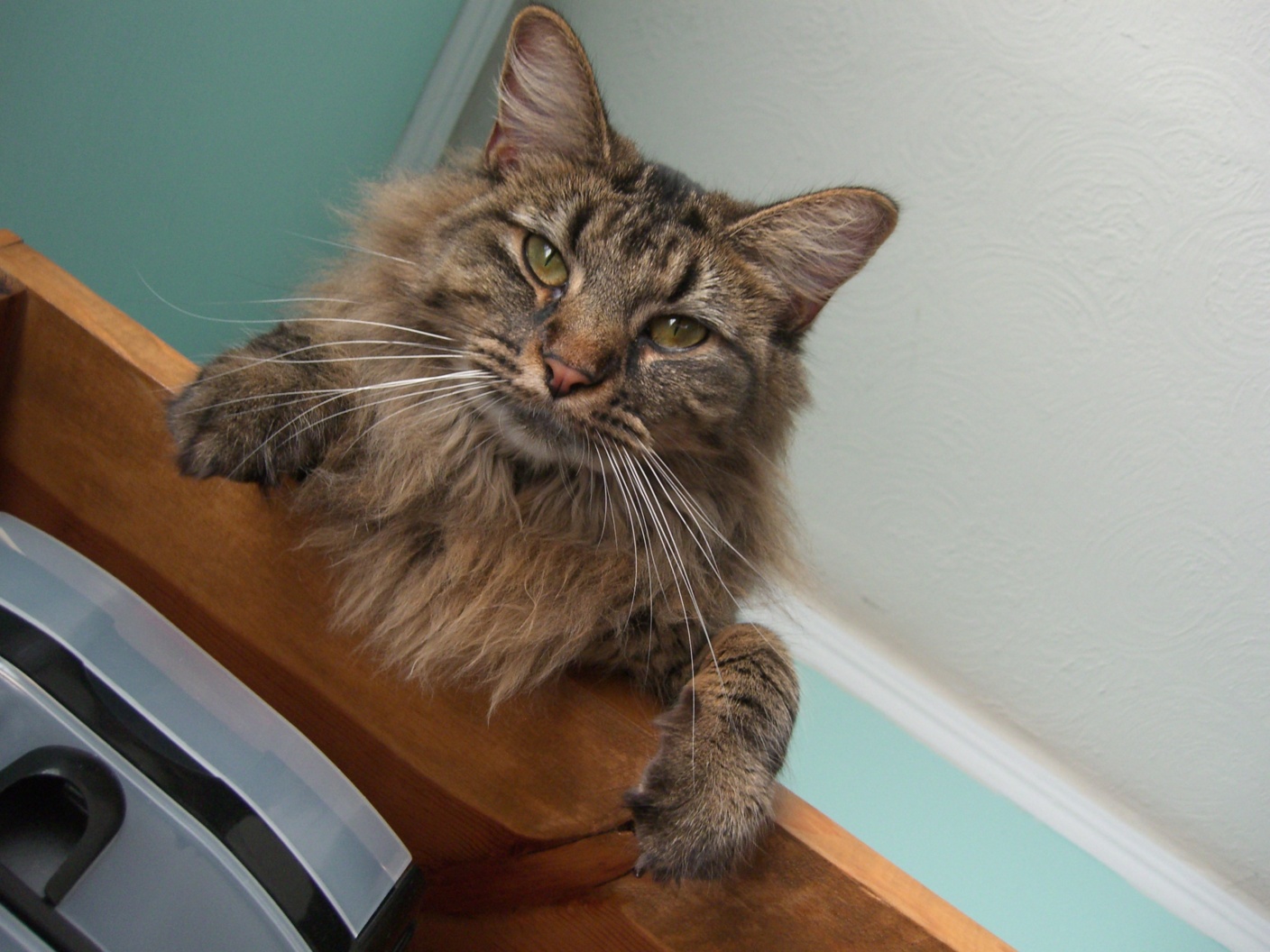
Cat
Nutmeg the Cat
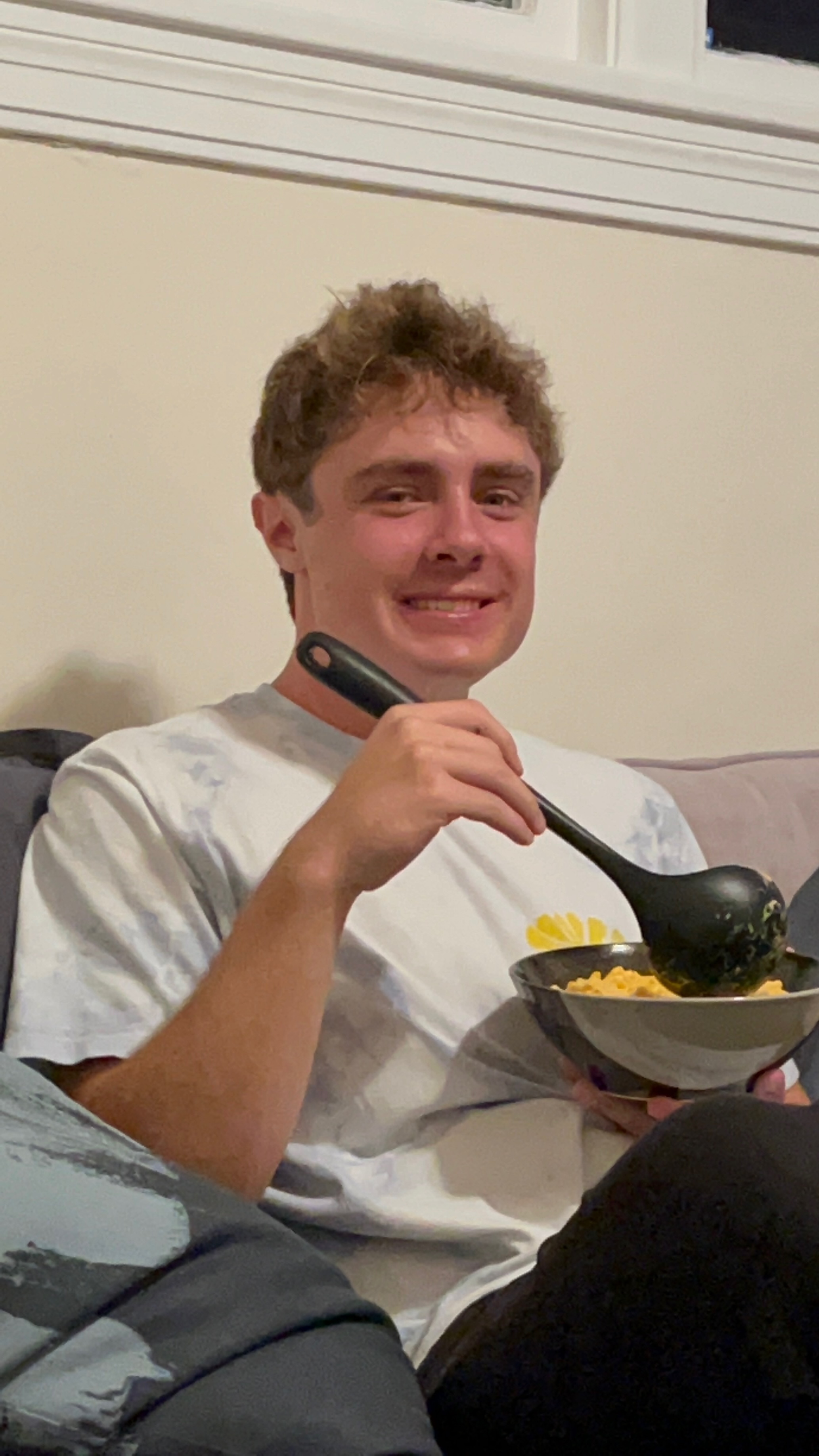
Human
Derek the Human
Hybrid Image
Hybrid Image
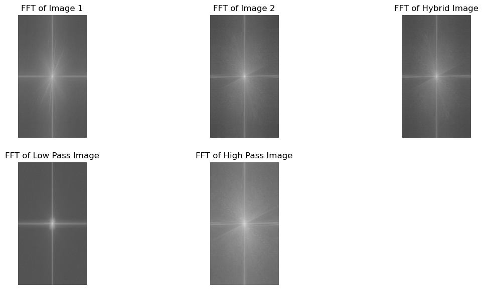
We can visualize the frequency response of these images by taking the Fourier Transform of the images and plotting the magnitude of the Fourier Transform. As we can see in these plots of the magnitude of the Fourier Transform, we only keep the low frequency portions of image 1 and the high frequency portions of image 2 to create the hybrid image.
Hybrid Image Fourier Transform
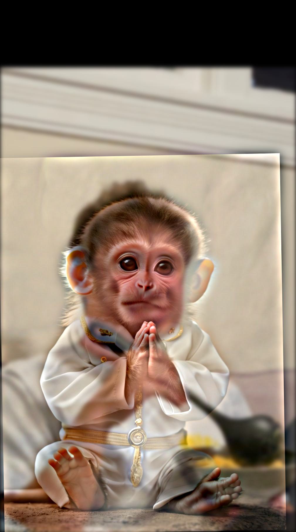
Hybrid Image Fourier Transform (for Miles-Monkey Hybrid)
Here are some other examples of hybrid images:
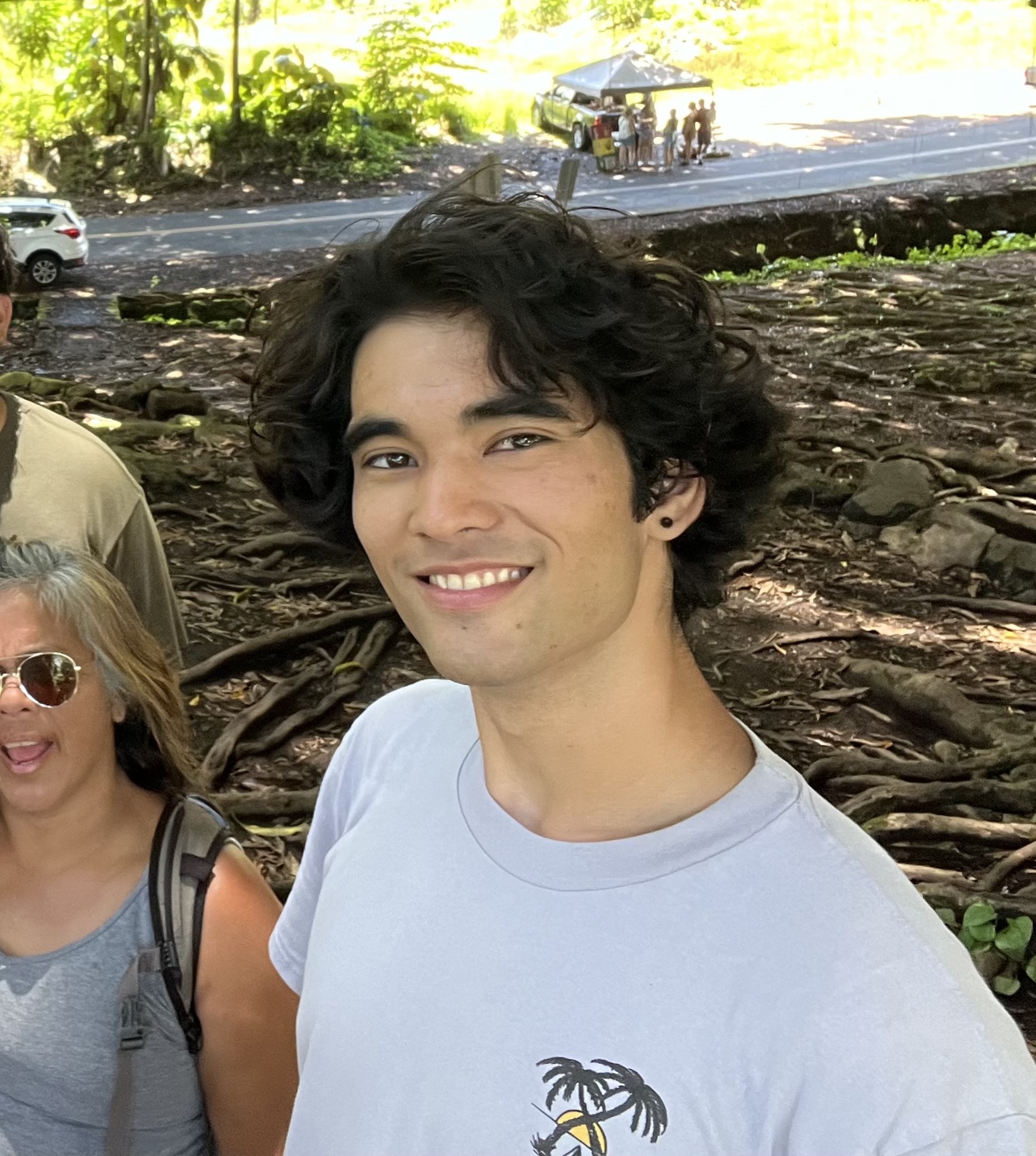
Image of My Roomate
Miles (my roomate)
Image of a Monkey
Monkey
Miles-Monkey Hybrid
Miles-Monkey Hybrid Image
Image of Dominic
Dom (old roomate)
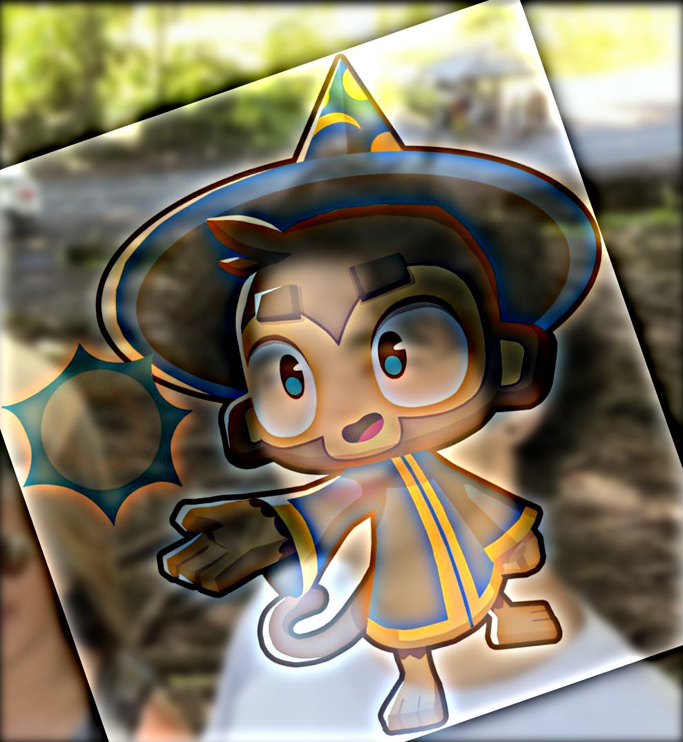
Image of Wizard Monkey
Wizard Monkey
Dom-Wizard Hybrid
Dom-Wizard Hybrid Image
This last image did not turn out great. I believe this was mostly because the shapes and color schemes of the two images were a little bit too off. It ended up only really looking like one image with a slight ghost of the other image.

Multi-resolution Blending

Introduction:

Another common task in image processing is to blend two images together. If we just did so by simply splicing the two pictures together, we would end up with a sharp line between the two images. We can improve this by using multiresolution blending to smooth out this seam between the two images. This is done by blending the two images at different resolutions and then combining them together.

Gaussian and Laplacian Stacks

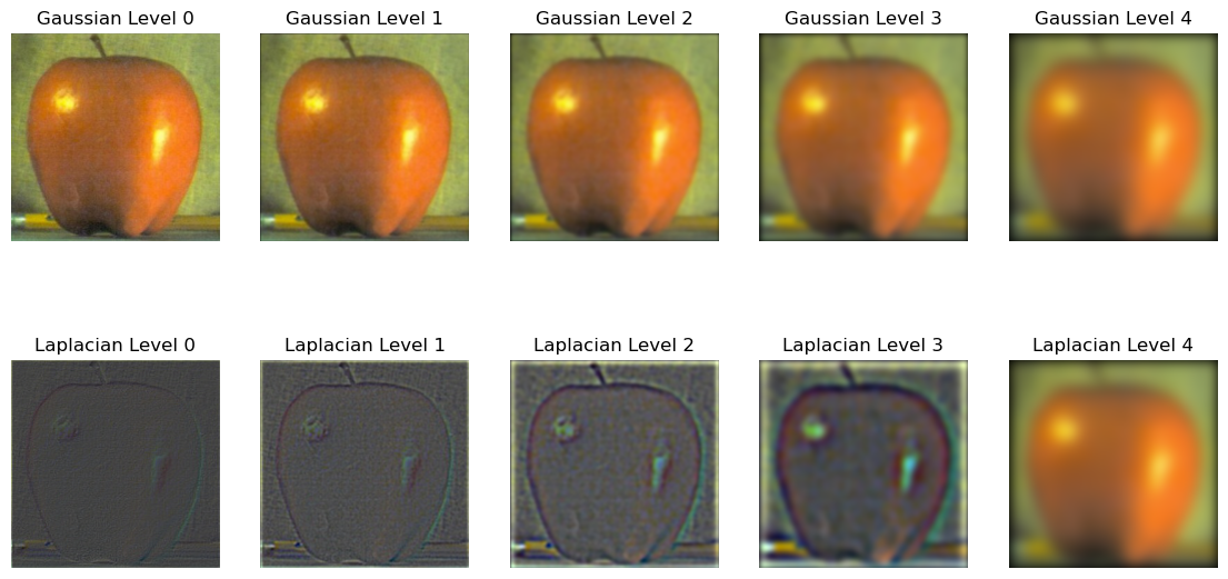
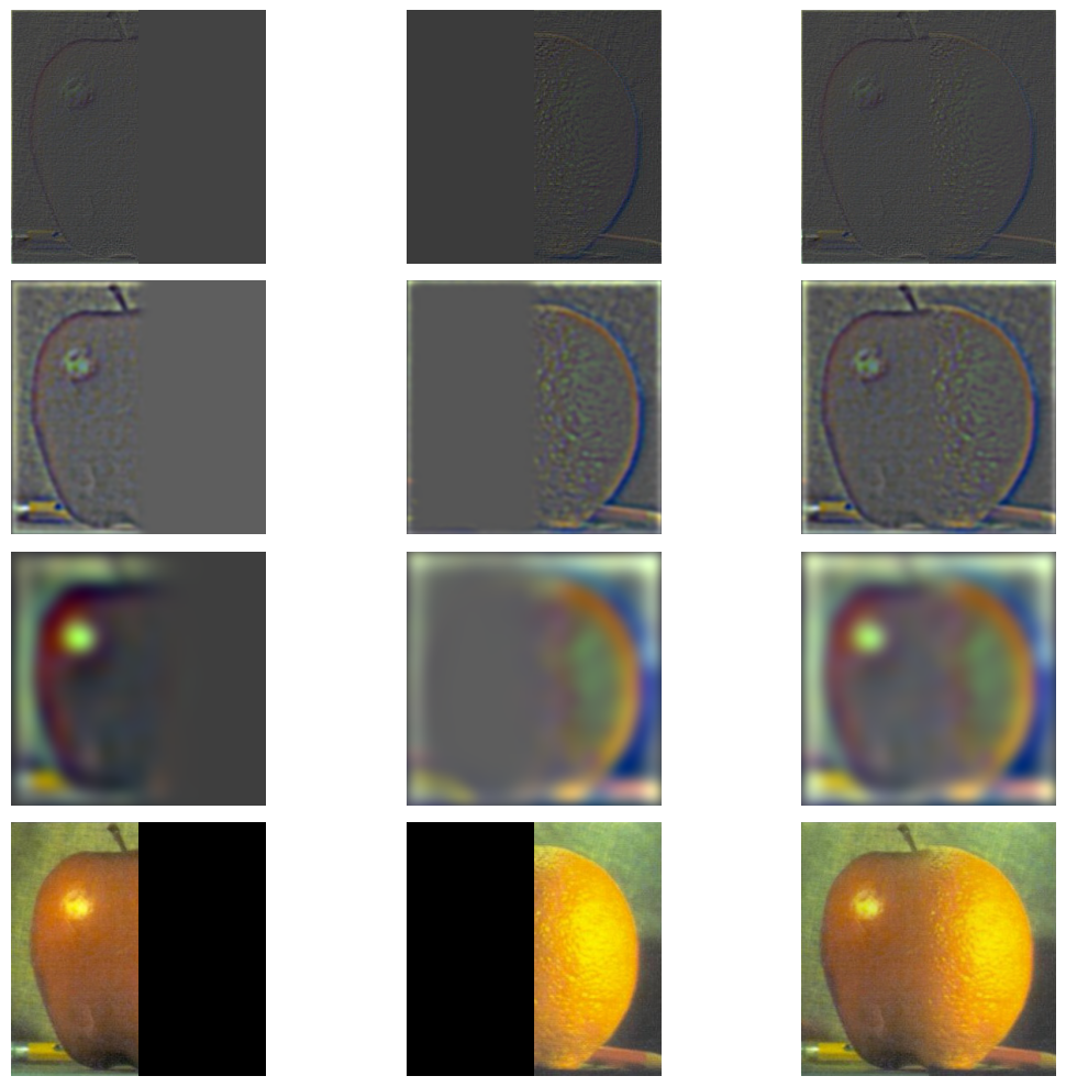
In order to separate our images into different resolutions, we use Gaussian and Laplacian Stacks. These breakdown our images into different frequency resolutions which we can then use later to combine together. Unlike the Gaussian pyramid we created in project 1, we can create a Gaussian Stack by simply applying a Gaussian kernel with increasing sigma values to the image. We can similarly get the Laplacian Stack by subtracting the different levels of the Gaussian stack. Here is our visualized Gaussian and Laplacian stacks for an apple:
Apple
Gaussian and Laplacian Stacks of an Apple

Implementing Multi-resolution Blending

Following the method described in the paper by Burt and Adelson, we can blend two images together by first creating the Gaussian and Laplacian stacks for both images. We also applied a Gaussian Stack to the mask in order to resolve the jagged edges of a simple spline We also applied a Gaussian Stack to the mask in order to resolve the jagged edges of a simple spline blend.
Image of Multiresolution Blending Process
Multiresolution Blending Process
Here are my results from blending two images together:
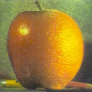
Oraple Blending
Oraple Blending Process
Oraple
Oraple
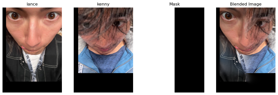
Lance-Kenny Blending
Lance-Kenny Blending Process
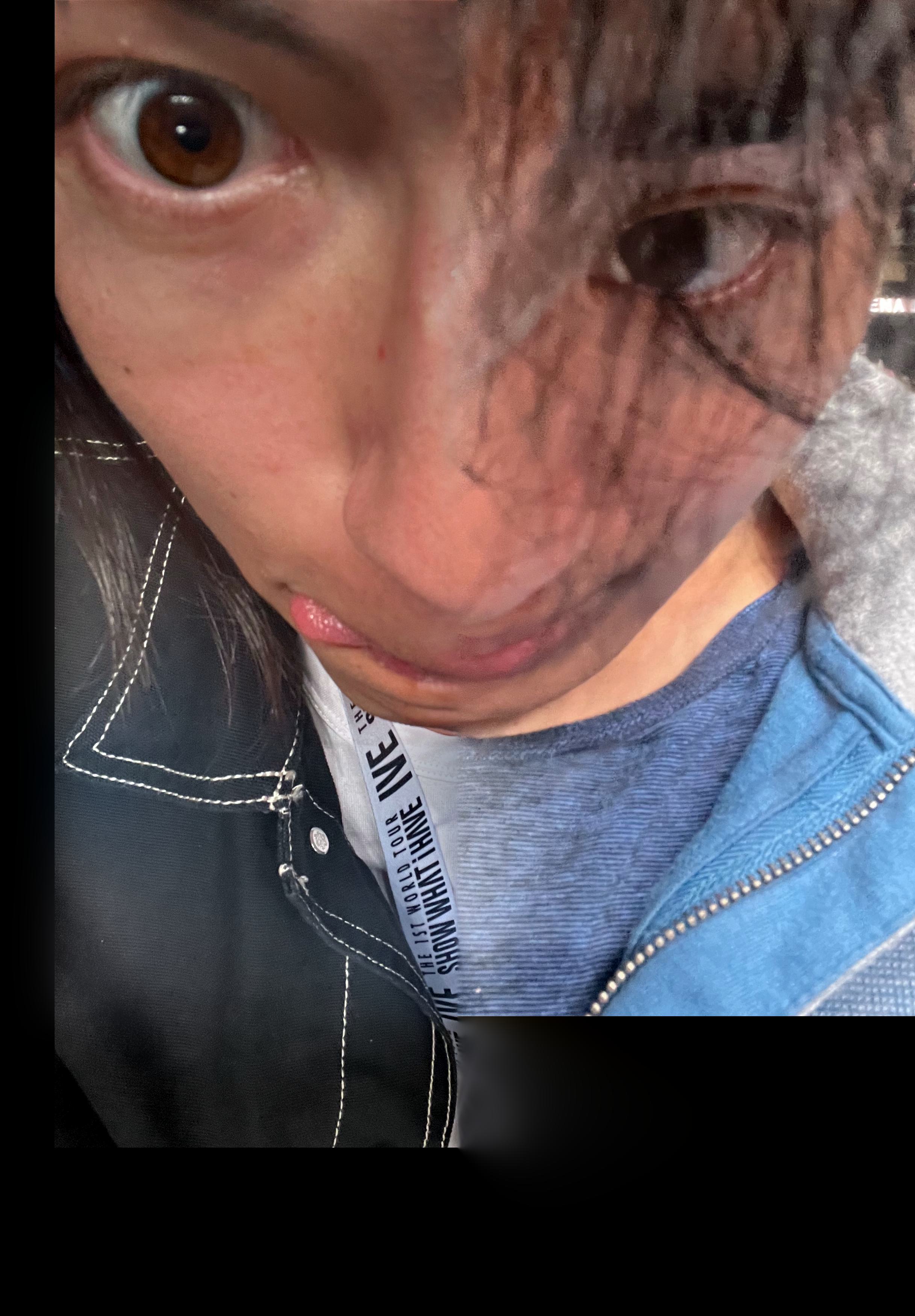
Lance-Kenny
Lance-Kenny
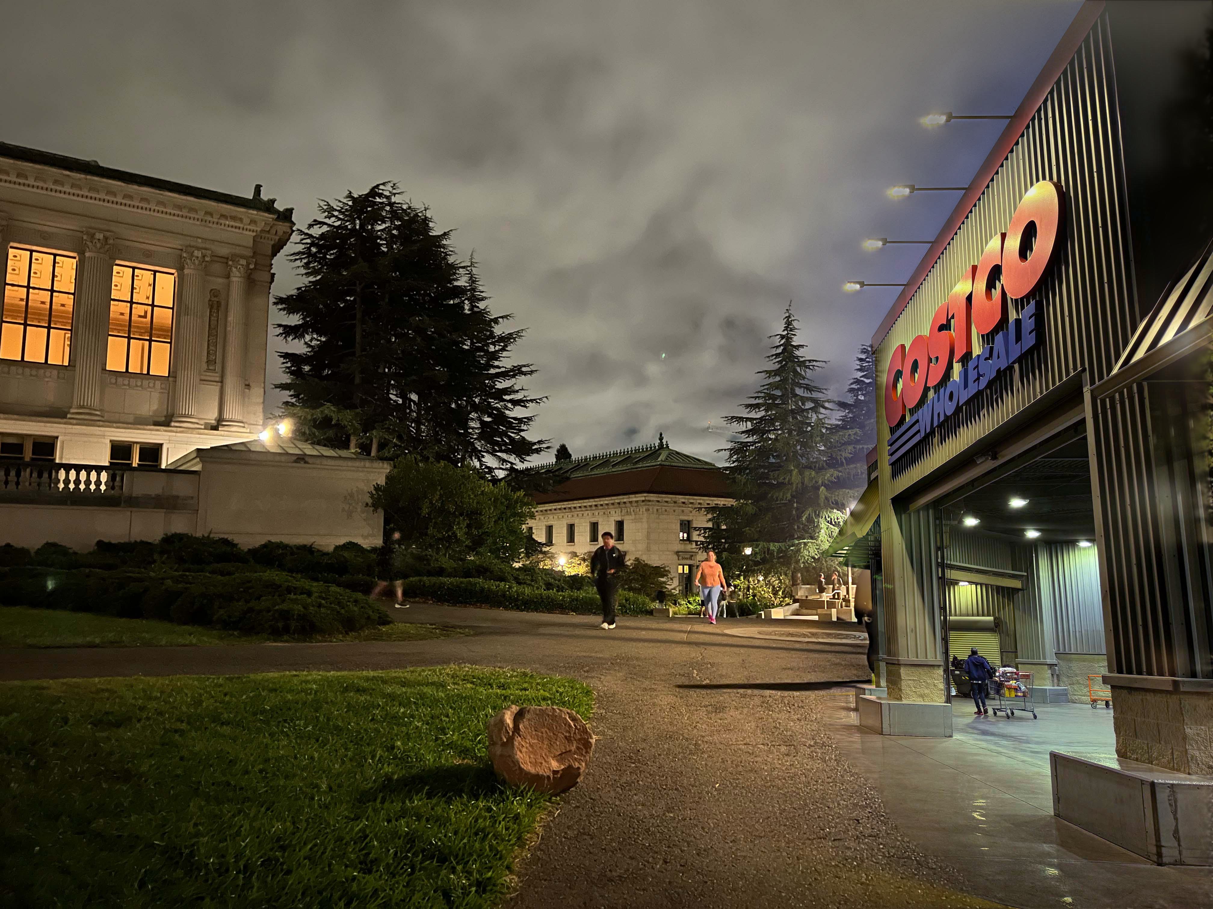
Costco Glade Blending Process
Costco-Glade Blending Process
Costco-Glade
Costco-Glade
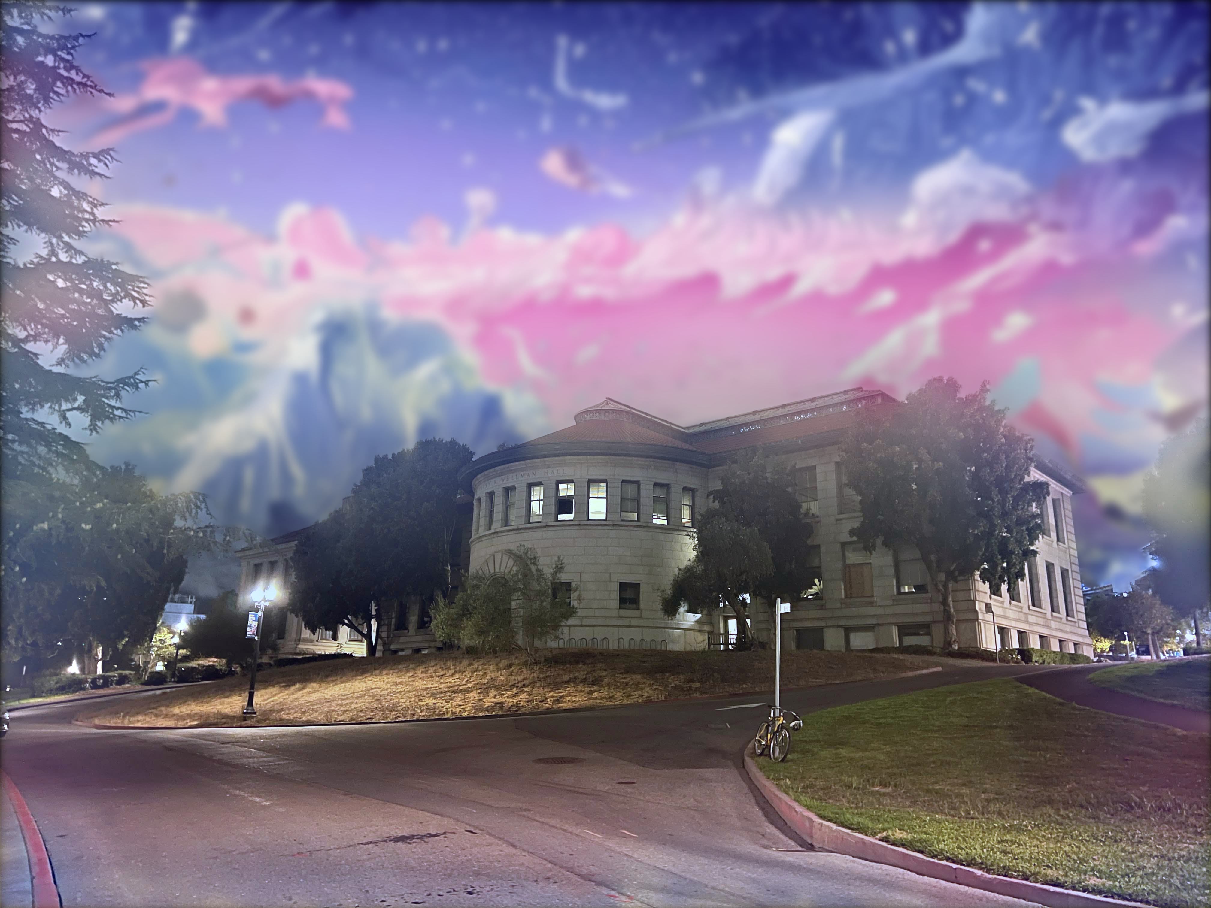
Wellman-Fantasy-Sky Blending Process
Dark Wellman Bright Sky Blending Process
Wellman-Fantasy-Sky
Dark Wellman Bright Sky
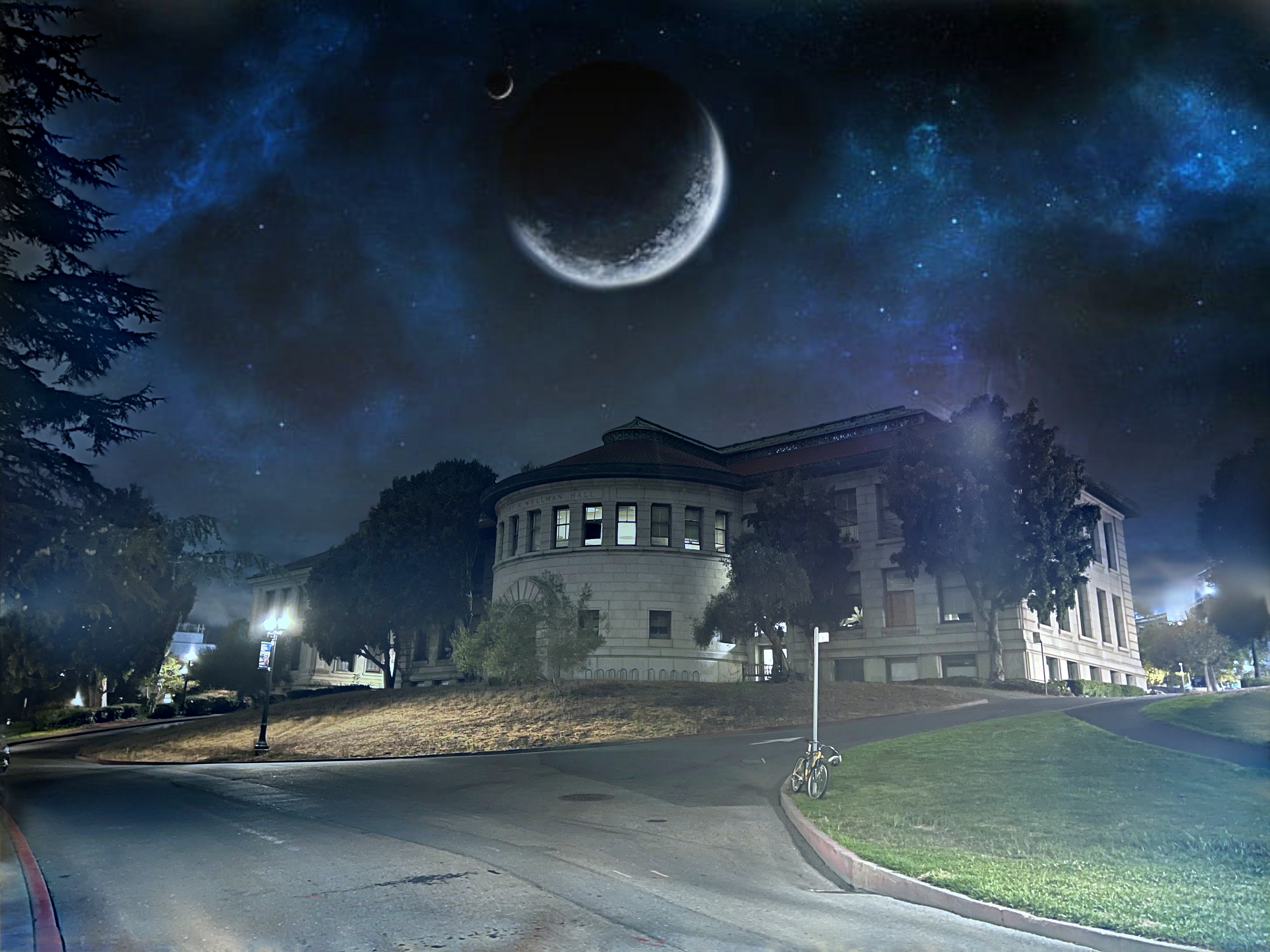
Dark-Wellman-Dark-Sky Blending Process
Dark-Wellman-Dark-Sky
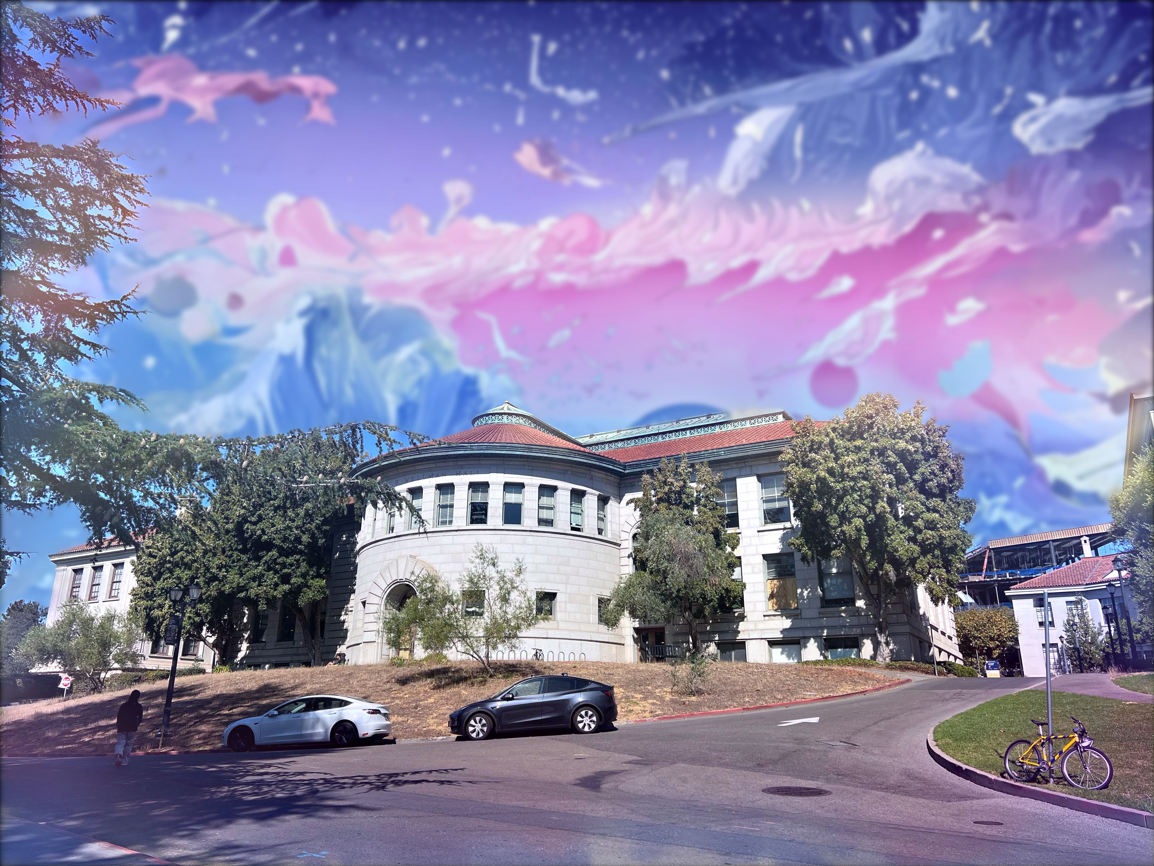
Bright-Wellman-Fantasy-Sky Blending Process
Bright-Wellman-Fantasy-Sky

Takeaways:

In this process, after blending together images with a basic vertical mask, I initially wanted to insert an object into an image with an irregular mask. However, as seen above, this didn't work out too well due to the differing colors in the images and the different FOV of the pictures. I then tried just blending the sky. However, this also looked slightly irregular due to the differing colors of my desired sky and the shadows of the image. Finally, I used different shaded skies to blend with the building, which I was able to blend together successfully. Another thing to note was that I created my irregular masks by drawing them by hand in photoshop. The jagged edges in these masks were unnoticeable in the final image because of the Gaussian blurring process of the mask. For this project overall, my main takeaways were how even simple operations can be used to seriously enhance images. Although I assume more complex operations can be used for better results, I was decently happy with the results I got from the simple operations I used. I found it quite cool and interesting all that I could do by just convolving images with a Gaussian kernel.