Part 1: Fitting a Neural Field to a 2D Image
In the first part, of this project, I started by developing my understanding of Neural Fields by implementing a 2D version of the model. The goal of this part was to fit a Neural Field to 2D images where we do not need to worry about radiance. Our system simplifies down to just having to implement a filed \(F: \{u, v\} \rightarrow \{r, g, b\}\) that maps 2D pixel coordinates to RGB values. We can do this by using a Multilayer Perceptron (MLP) network with Sinusoidal Positional Encoding (PE) that takes in a two dimensional input and outputs a three dimensional value (pixel color).
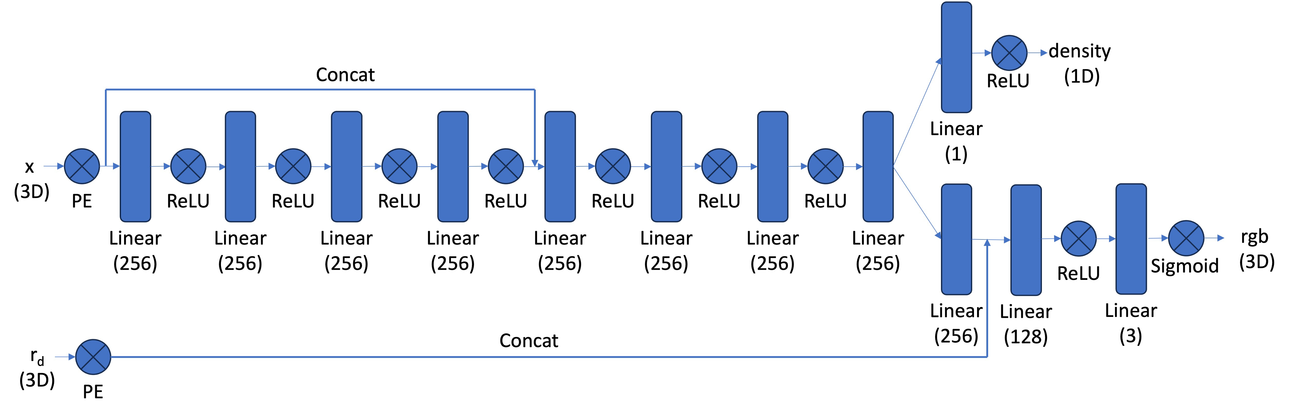
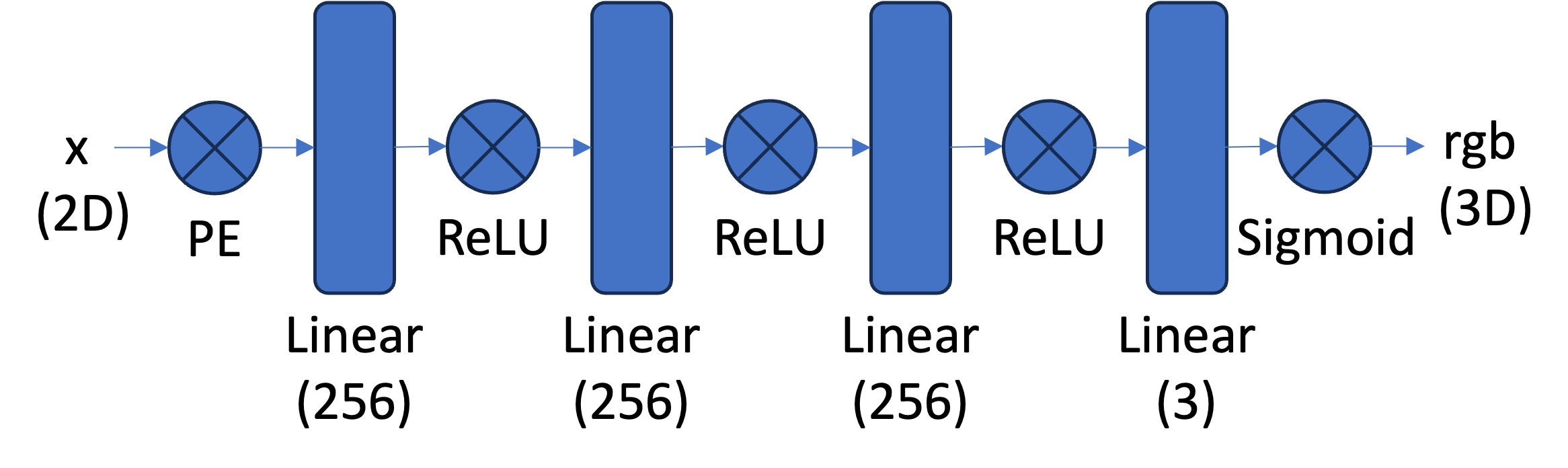
Model Architecture:
The network is composed of a couple fully connected layers followed by a ReLU activation function. One of the more interesting parts of this model architecture is the use of the Sinusoidal Positional Encoding (PE). This is an operation you apply to the input that expands the dimensionality of the input by adding sinusoidal functions of different frequencies. This allows the model to learn higher frequency patterns in the data based on the max frequency level \(l\) we choose. \[ PE(x) = \{x, \sin(2^0\pi x), \cos(2^0\pi x), \sin(2^1\pi x), \cos(2^1\pi x), \ldots, \sin(2^{L-1}\pi x), \cos(2^{L-1}\pi x)\} \]
Our overall architecture is as follows: (we use a Sigmoid activation at the function to constrain our output range to \((0, 1)\) to match valid pixel colors.)
Dataloader
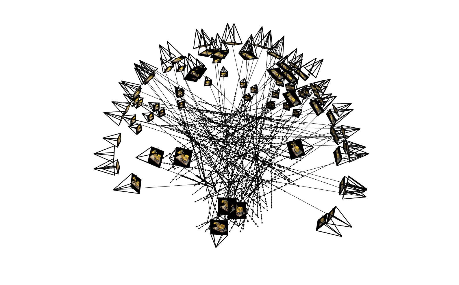
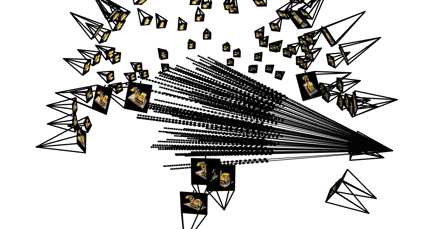
The first step in our process of training our 2D Neural Field is to generate data to train on. Since the images we want to work with are a little bit too high resolution to train with all of our pixels, we randomly sample \(N\) pixels from our image during every training iteration. We can do this all within our dataloader, which will return both the \((N \times 2)\) pixel coordinates and the corresponding \((N \times 3)\) RGB values of the pixels. These will be our inputs and supervision targets to our model we will use to train. We will also normalize both of these values before inputting them into our model.
Training
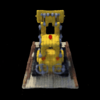
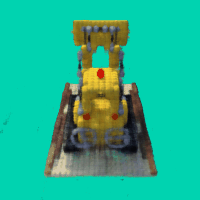
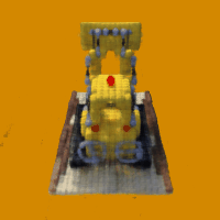
We will train our model using the mean squared error (MSE) loss function and an Adam optimizer with learning rate \(0.01\). We will run our model for \(2000\) iterations with a batch size of \(10,000\) and a max frequency level of \(L=10\). Also, instead of using the MSE as our metric, we will display the Peak Signal-to-Noise Ratio (PSNR) of our model's output compared to the ground truth image. This is the more common metric used for measuring reconstruction quality of an image, and easy to calculate from the MSE. If an image is normalized to \([0, 1]\), then the PSNR is simply: \[ PSNR = 10 \cdot \log_{10}\left(\frac{1}{\text{MSE}}\right) \] Here are the results of our initial training, with visualizations of the model's output during different stages of training.

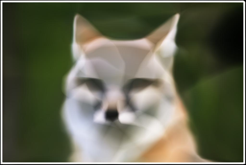
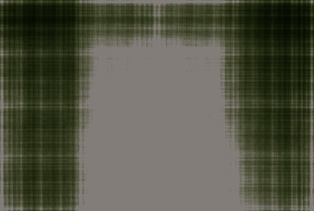
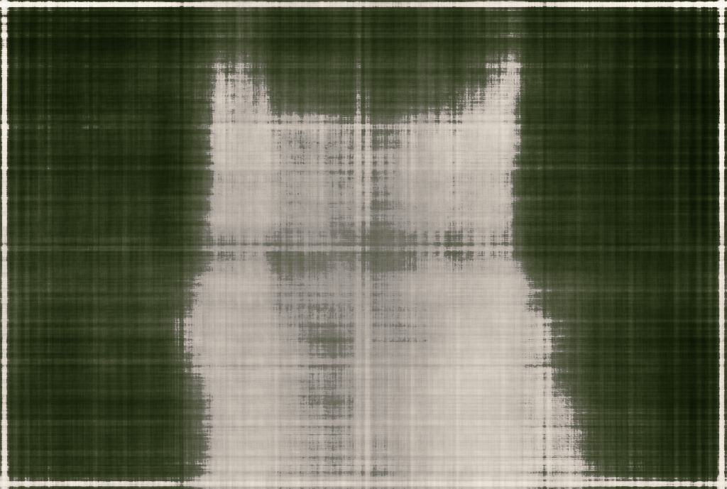
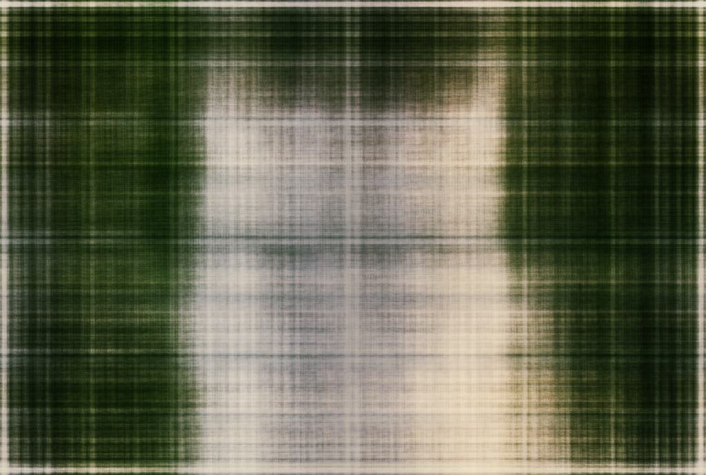
Iteration 0
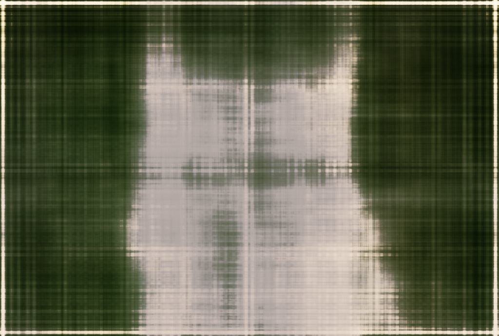
Iteration 50
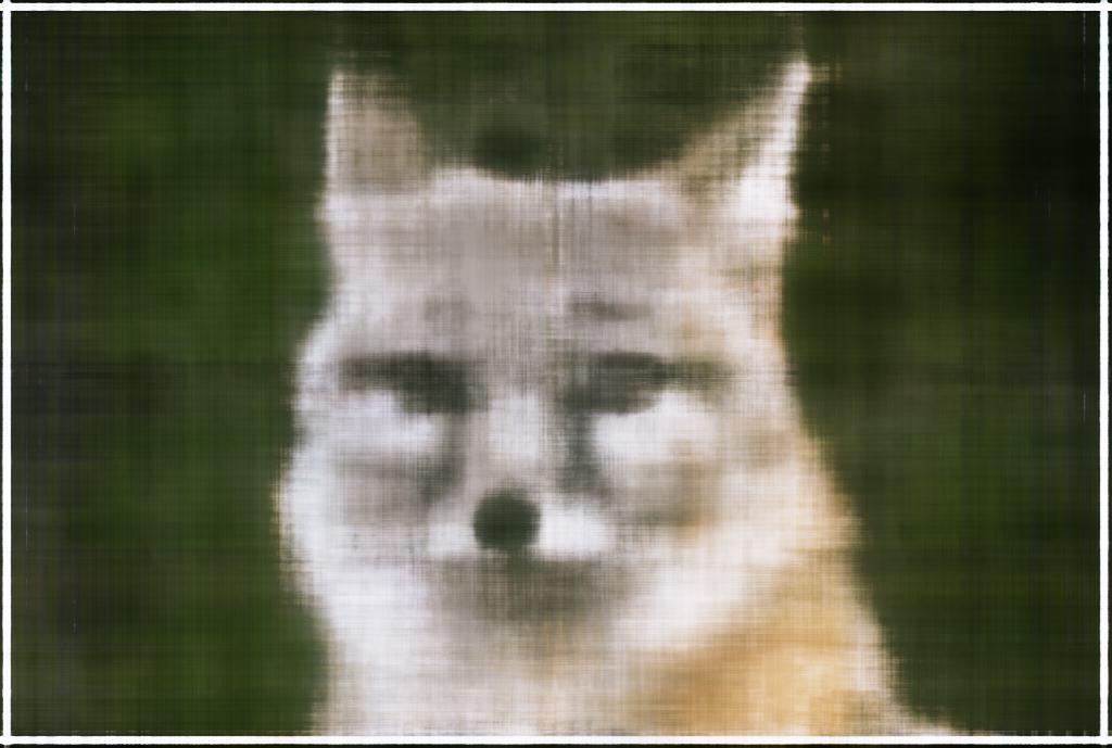
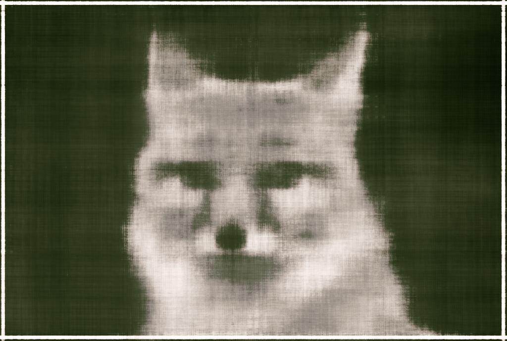
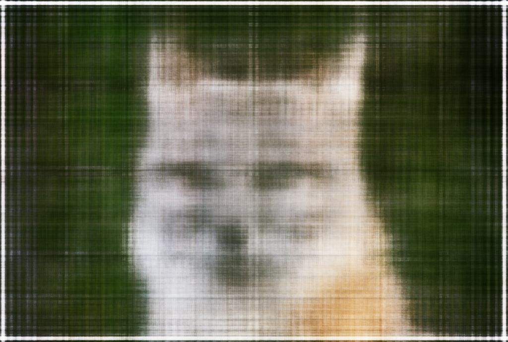
Iteration 100
Iteration 200
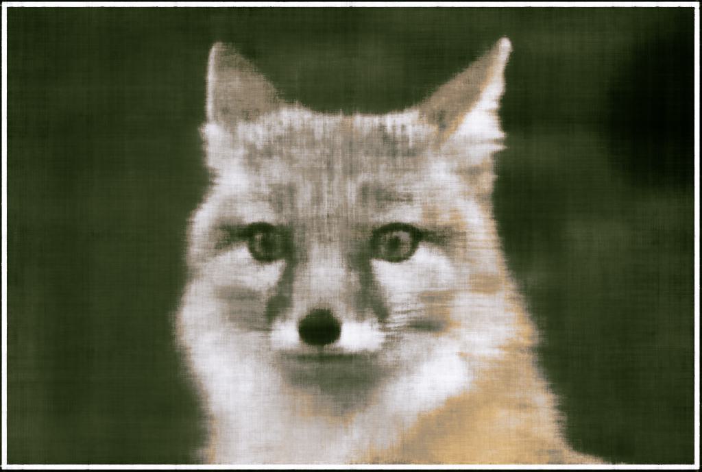
Iteration 500

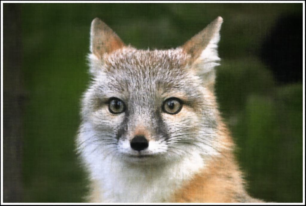
Iteration 1000
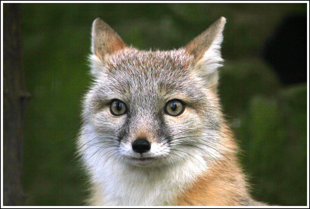
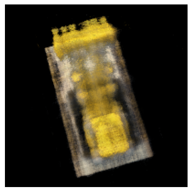
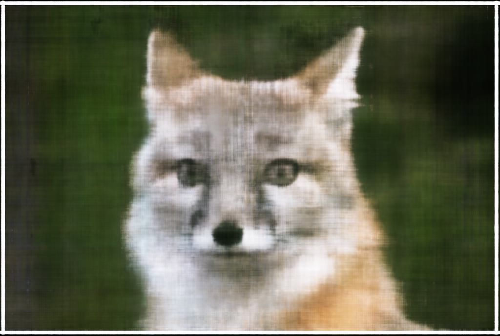
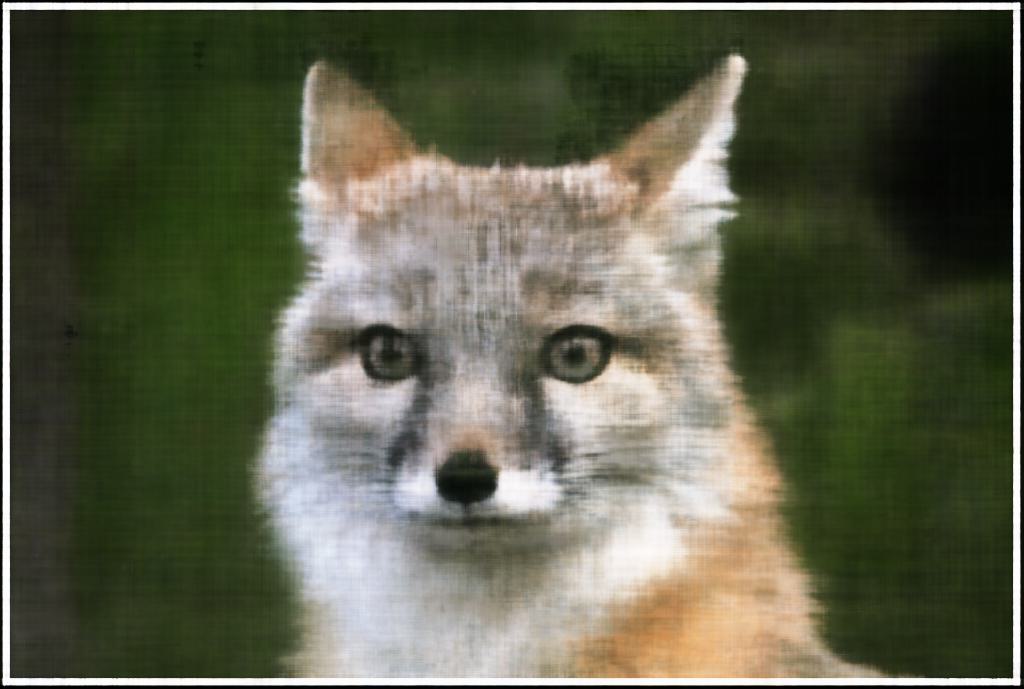
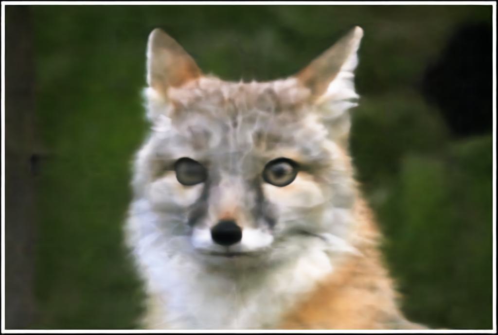
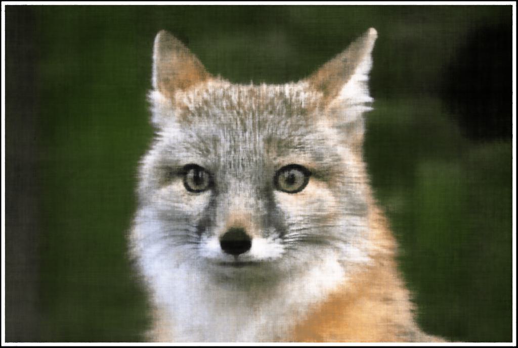
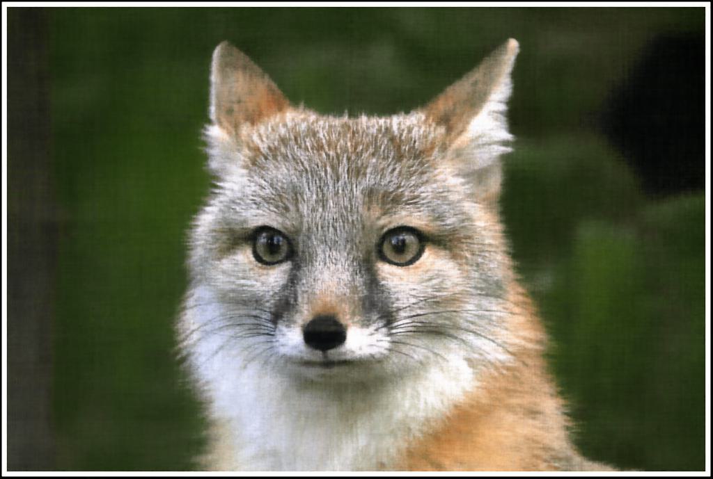
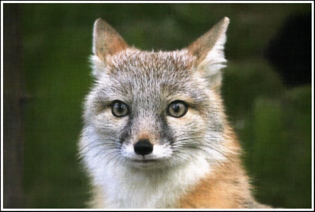
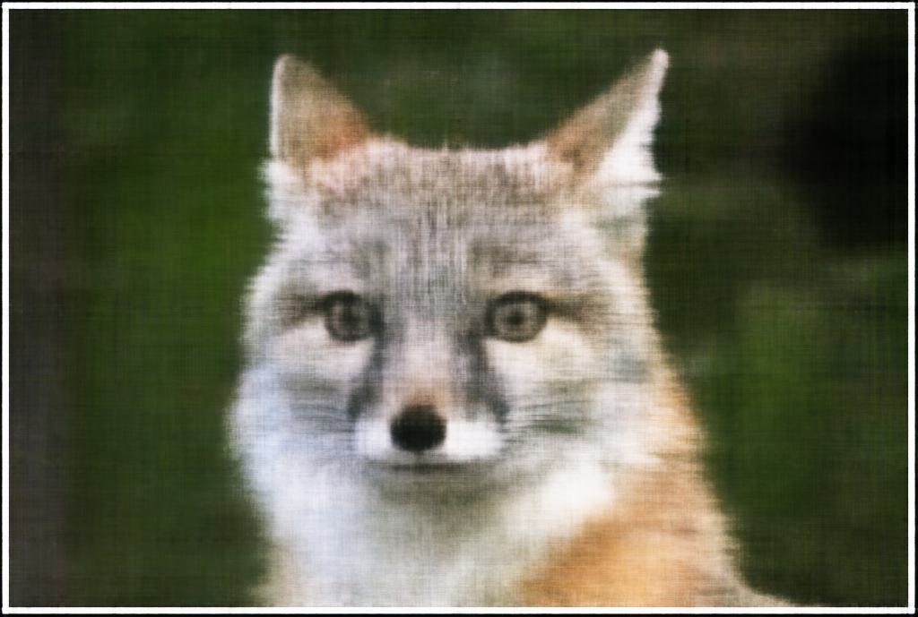
Original Image
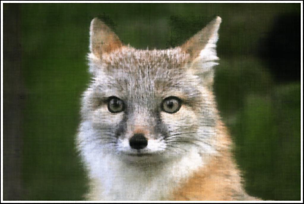
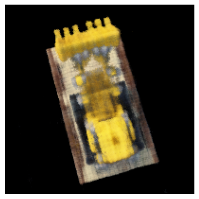
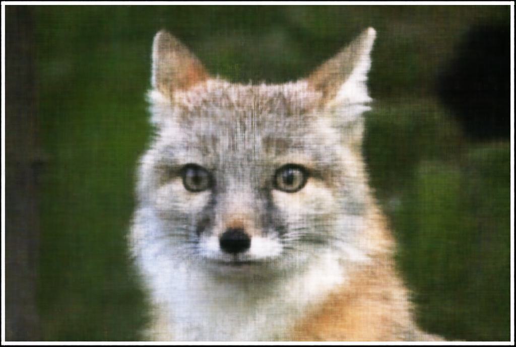
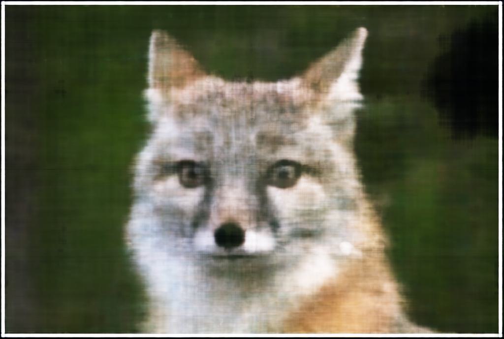
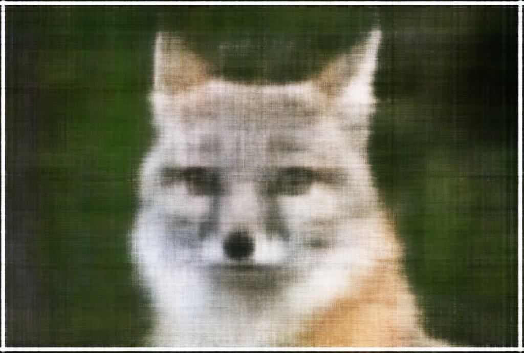
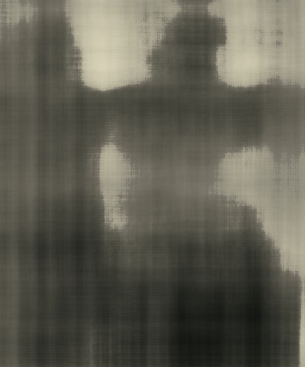
Final Output, PSNR = 26.325
As we can see, our model is able to learn the underlying structure of the image and produce a reasonable reconstruction of the image. The PSNR of our final output is \(26.325\), which is a decent reconstruction of the image.
Hyperparameter Tuning
We can better understand how our model works by adjusting the hyperparameters of our model. We can try to see how the model performs with different max frequency levels, different numbers of layers, and different numbers of neurons in each layer. While our image reconstruction was quite good, we can also use hyperparameter tuning to attempt to get a better image reconstruction.
Max Frequency Level:
The max frequency level in our model corresponds to the dimensionality of our positional encoding. I tested decreasing the max frequency levels to see the effects of adjusting the dimensionality of our input. As seen in the following images, the model is able to learn the underlying structure of the image with lower frequency levels, but the details are clearly left out of the image without a high enough max frequency level.
L = 1, PSNR = 23.366
L = 5, PSNR = 25.366
L = 10, PSNR = 26.325
Number of Hidden Layers
In a Multilayer Perceptron model, we have a bunch of fully connected layers that are connected to each other through activation functions. The first fully connected layer is the inpuit layer, the last is the output layer, and all of the others in between are known as hidden layers. Our initial architecture had \(2\) hidden layers, but we can try to adjust the number of layers to determine how that affects our model's performance.
1 Hidden Layer, PSNR = 25.346
2 Hidden Layers, PSNR = 26.325
5 Hidden Layers, PSNR = 27.776
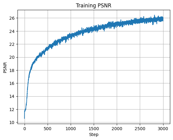
We can see that with more hidden layers, our model becomes more complex and is better able to learn our input image. However, one thing to note is that with more hidden layers, there is more to learn, and I had to increase the number of iterations and decrease the learning rate to get the model to begin to converge. Here is our best model with \(10\) hidden layers, a learning rate of \(0.001\), and \(3000\) iterations which achieved a PSNR of \(28.189\):
Iteration 50
Iteration 100
Iteration 200
Iteration 500
Iteration 1000
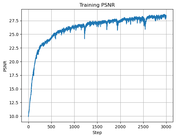
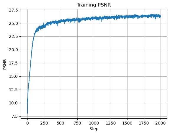
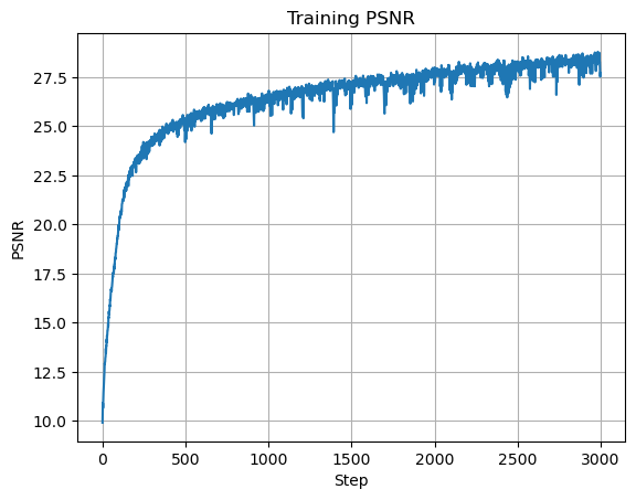
Plot of Training PSNR
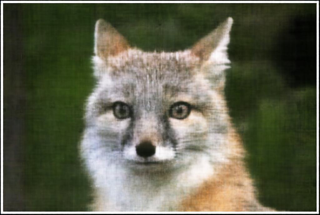
Final Output, PSNR = 28.189
Number of Hidden Units
The number of hidden units in a layer is the number of neurons in that layer, or the number of parameters that the model can learn. We can adjust the number of hidden units to see how that affects our model's performance. In our original model, we used \(256\) hidden units in each layer, but we can try to adjust this number to see how it affects our model's performance.
64 Hidden Units, PSNR = 24.8
128 Hidden Units, PSNR = 25.626
256 Hidden Units, PSNR = 26.325
400 Hidden Units, PSNR = 27.936
Similarly to the number of hidden layers, I also had to decrease the laerning rate and increase the number of iterations in order to get the model loss to converge (I used a learning rate of \(0.001\) and \(3000\) iterations to train all of these models). This is once again because increasing the number of hidden units increases the complexity of our model, and thus requires more iterations to learn the underlying structure of the image. We can see that increasing the number of hidden units allows the model to perform better. Here is my best model which used \(512\) hidden units and achieved a PSNR of \(27.696\):
Iteration 50
Iteration 100
Iteration 200
Iteration 500
Iteration 1000
Plot of Training PSNR

Final Output, PSNR = 27.696
Conclusion
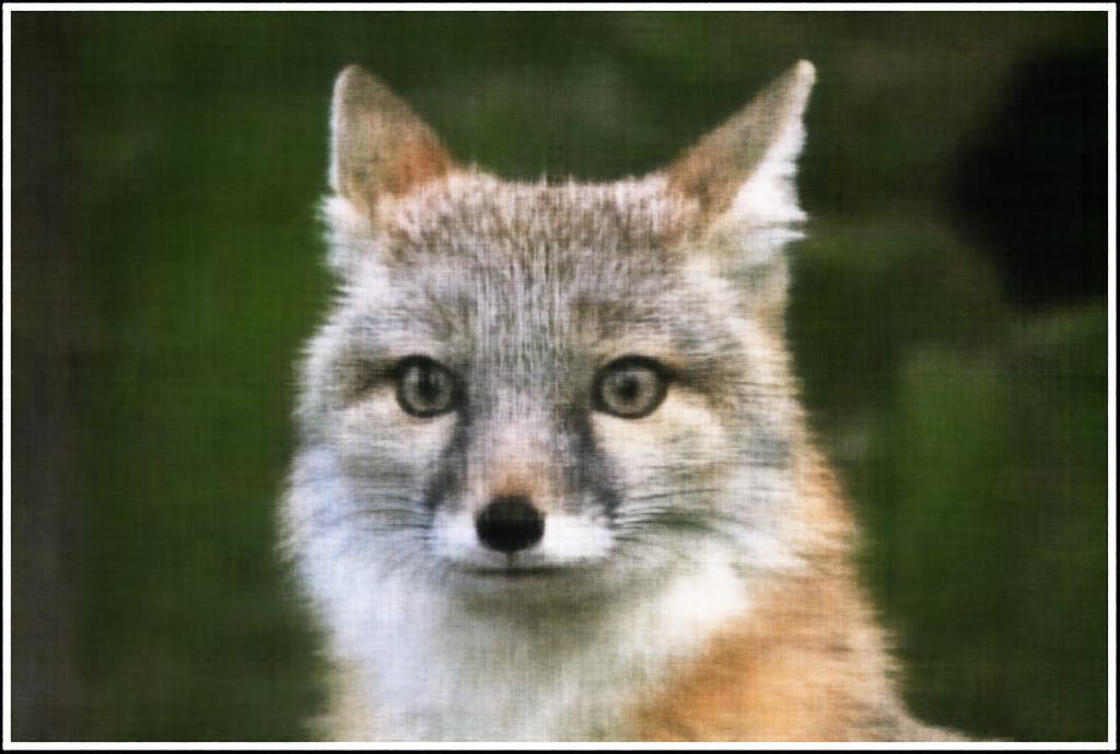
From this hyperparameter testing, we can see that increasing the max frequency level, the number of hidden layers, and number of hidden units all help to improve the model's ability to reconstruct the image. However, these all come with tradeoffs, as epecially for the latter two, increasing the model complexity increases the training time. Taking this into account, I decided on the configuration of a max frequency level of \(10\), \(7\) hidden layers, and \(512\) hidden units with a learning rate of \(0.001\) and \(3000\) iterations to try our model on another image:

Iteration 0
Iteration 50
Iteration 100
Iteration 200

Iteration 500

Iteration 1000
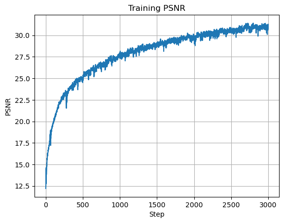
Plot of Training PSNR

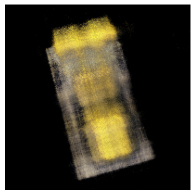
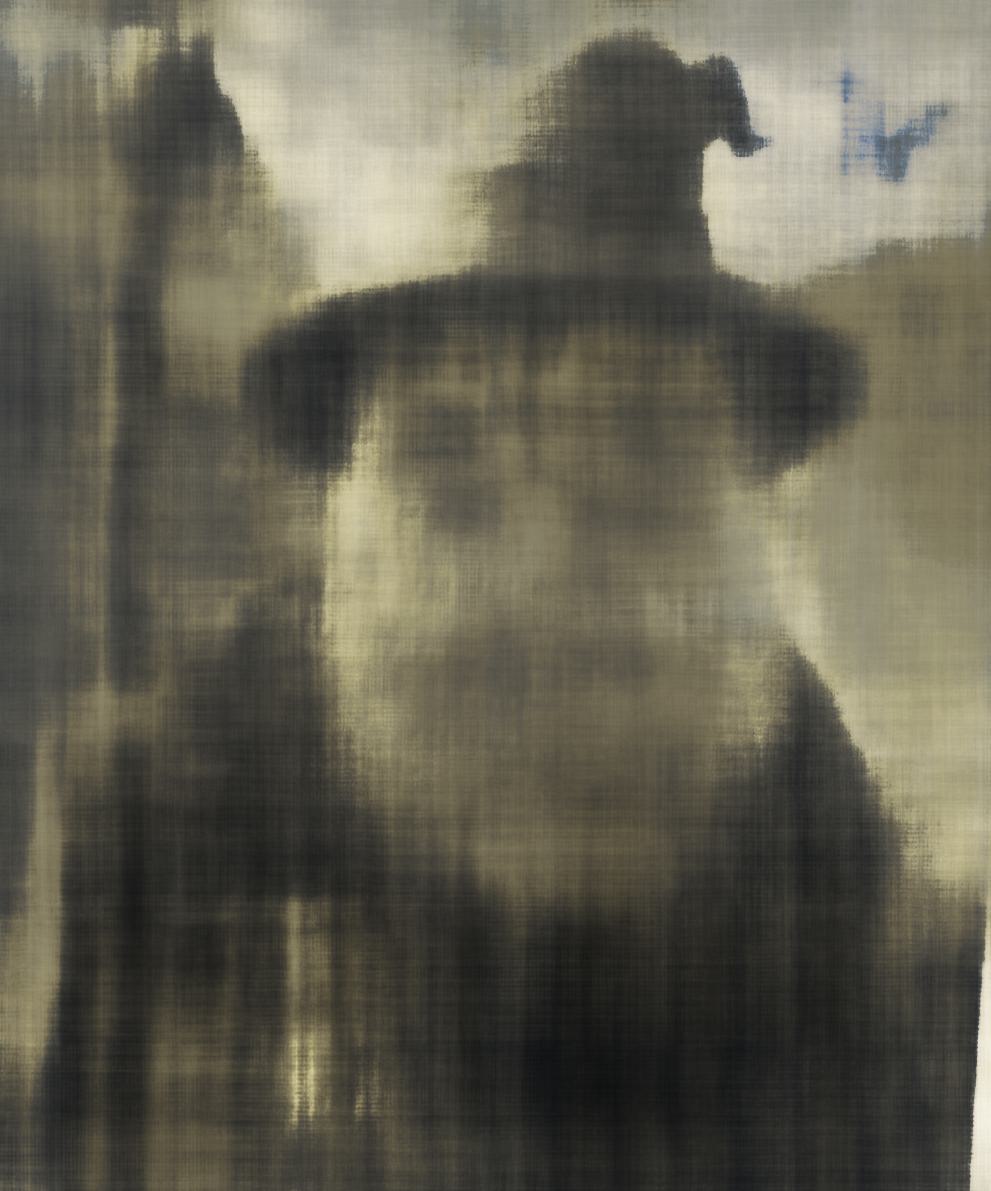
Final Output, PSNR = 30.798

Original Image